重磅独家 | 腾讯AI Lab AAAI18现场陈述论文：用随机象限性消极下降算法训练L1范数约束模型

前言：腾讯 AI Lab共有12篇论文入选在美国新奥尔良举行的国际人工智能领域顶级学术会议 AAAI 2018。腾讯技术工程官方号独家编译了论文《用随机象限性消极下降算法训练L1范数约束模型》（Training L1-Regularized Models with Orthant-Wise Passive Descent Algorithms），该论文被 AAAI 2018录用为现场陈述论文（Oral Presentation），由腾讯 AI Lab独立完成，作者为王倪剑桥。

L1范数约束模型是一种常用的高维数据的分析方法。对于现代大规模互联网数据上的该模型，研究其优化算法可以提高其收敛速度，进而在有限时间内显著其模型准确率，或者降低对服务器资源的依赖。经典的随机梯度下降 (SGD) 虽然可以适用神经网络等多种模型，但对于L1范数不可导性并不适用。

在本文中，我们提出了一种新的随机优化方法，随机象限性消极下降算法 (OPDA)。本算法的出发点是L1范数函数在任何一个象限内是连续可导的，因此，模型的参数在每一次更新之后被投影到上一次迭代时所在的象限。我们使用随机方差缩减梯度 (SVRG) 方法产生梯度方向，并结合伪牛顿法 (Quasi-Newton) 来使用损失函数的二阶信息。我们提出了一种新的象限投影方法，使得该算法收敛于一个更加稀疏的最优点。我们在理论上证明了，在强凸和光滑的损失函数上，该算法可以线性收敛。在RCV1等典型稀疏数据集上，我们测试了不同参数下L1/L2范数约束Logistic回归下该算法性能，其结果显著超越了已有的线性收敛算法Proximal-SVRG，并且在卷积神经网络 (CNN) 的实验上超越Proximal-SGD等算法，证明了该算法在凸函数和非凸函数上均有很好的表现。

Hello, everyone, I am Jianqiao Wangni, from Tencent AI Lab.

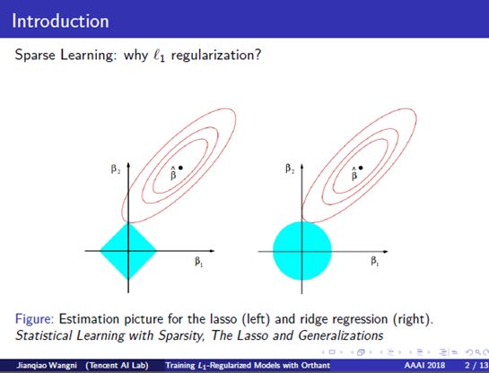
1. Introduction: Learning sparse representation has been a very important task for data analysis. For example, in biology, it usually involves millions of genes for the genetic analysis of a single individual. In finance series prediction, online advertising, there also lots of cases where the data numbers are even smaller than data dimensions, which is an ill-conditioned problem without the sparse prior. So, for the conventional models, like logistic regression and linear regression, we put an L1 norm regularization, which is the sum of absolute values, to build robust applications with high dimensional data. And they are very powerful for learning sparse representations. To give an intuitive example. The blue areas are the constrained regions, L-1 norm ball on the left and L-2 norm ball on the right, respectively, while the red circles are the contours of the average of square loss functions. The intersection point between the balls and the contours are the solution to such regularized models. We can see that the solution to the L1-regularized model is near the Y-axis, which means that the X-dimension element is more approaching zero.

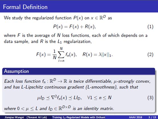
2. Formal Definition: Now we go to the analytical part. We study a regularized function P(x) which equals to F(x) + R(x), where F(x) is the average of N loss functions each of which depends on a data sample, and R is the L_1 regularization. We also assume that each loss function is twice differentiable, strongly convex and smooth, which are general assumptions in convex optimization. The L1 norm is not differentiable. One of most representative optimization method is the proximal method, which iteratively takes a gradient descent step and then solves a proximal problem on the current point.

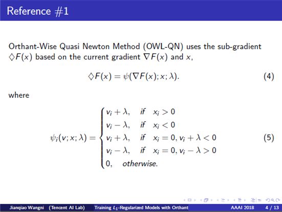
3. Reference 1: Our primary reference is the orthant-wise limited-memory quasi-newton method, OWL-QN, which was based on L-BFGS, a representative quasi-Newton method that overcame an obstacle that L1 norms are not differentiable. This method restricts the updated parameter to be within a certain orthant, because that in every single orthant, the absolute value function are actually differentiable. A key component of OWL-QN is about the subgradient on zero points. The subgradient of the L1 regularization R(x) can be whether positive lambda or negative lambda. Take the third branch for an example, we study a single dimension, I-th dimension, of the current point X_i and the gradient, V_i. If X_i equals to zero, and X_i plus lambda is negative, then the subgradient is set to be V_i plus positive lambda, since after subtracting this subgradient, X_i will be a positive value, then the subgradient of R(x) will still be positive lambda, this makes the subgradient of the L1 norm to be consistent across one iteration.

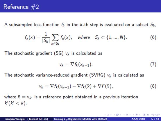
4. Reference 2: To process the massive internet data, many optimization methods were proposed to speed up the training process. The stochastic gradient descent method, SGD, is a popular choice for optimization. However, SGD generally needs a decreasing stepsize to converge, so it only has a sublinear convergence rate. Recently, some stochastic variance reduction methods, such as SVRG and SAGA, can converge without decreasing stepsizes and achieve linear convergence rates on smooth and strongly-convex models. In SGD, the descent direction in the k-th step, v_k, is evaluated on a stochastic subset S_k of the dataset. In SVRG, we need to periodically calculate a series of full gradients that depend on all data, on some reference points, say tilde-X. The full gradient constructs the third term of v_k of SVRG, then we have to balance the gradient in expectation, by subtracting a stochastic gradient on tilde-X, which is calculated on the same subset S_k.

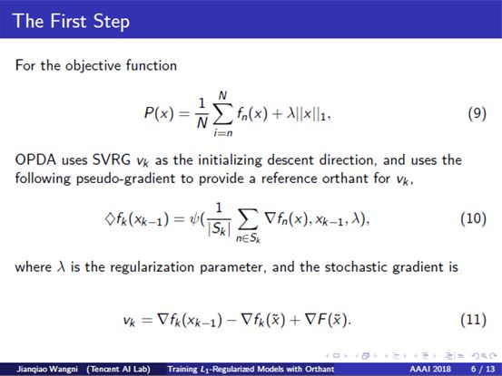
5. The First Step: Now we proceed to our method. Although being efficient, OWL-QN can be further improved, for examples, by dropping the line-search procedure, or using a stochastic gradient instead of the accurate but costly full gradient. Inspired by SVRG and OWL-QN, we develop a stochastic optimization method for in L1-regularized models. This is more complicated than the smooth function. At the first step, we calculate the SVRG of the loss function F(x), then we use an idea from OWL-QN to push the descent direction toward maintaining the same orthant after one iteration, and this will be used as a reference orthant. Our actual descent direction V_k is calculated as the third equation here.

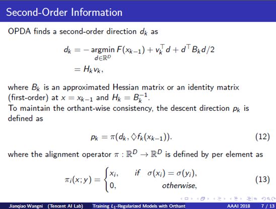
6. The Second-Order Information: At this point, we have an optional choice about the descent direction, we can use the second-order information of the loss function, by calculating the Hessian matrix on the current point, or estimating an approximated Hessian matrix, like quasi-Newton method. Then the descent direction D_k can be obtained by minimizing the following quadratic expansion around the current point. And if we use L-BFGS, we actually do not need to do the matrix inversion like the equation, this can be done through efficient matrix-vector multiplications. We may also directly assign V_k to D_k, as a typical first-order method. After this step, the orthant of the direction D_k has to be consistent with V_k, which means that, if some dimensions of D_k have different signs with V_k, they have to be aligned to zero, and we note the aligned version to be P_k.

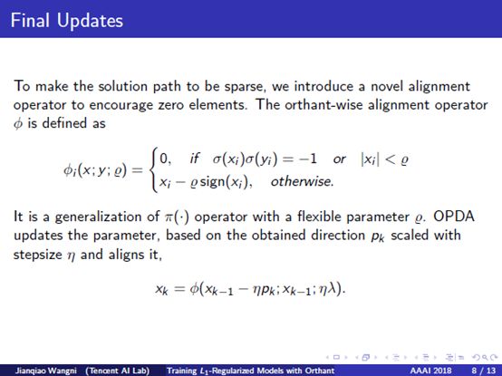
7. Final Updates: The aforementioned calculation does not explicitly involve the partial derivative of R(x), the L1 regularization, except for the alignment reference, since we are avoiding additional variance to the stochastic gradient. To make the solution to be sparse, we introduce a novel alignment operator to encourage zero elements, if X and Y had different signs, or the absolute value of X is less than a threshold, X would be forced to be zero. By this alignment operator, after each time we complete the previous calculation, we examine if the next point is in the same orthant as the current point, if not, some dimensions of the next point will be zero. After this step, clearly more dimensions of X_k should be zero instead of being small but nonzero values.

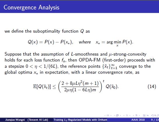
8. Convergence Analysis: In the paper, we prove that, under the assumption of smoothness and strong-convexity, our method will converge with a linear convergence rate. Due to lack of time, we do not use too much time on details of this heavy mathematical analysis.

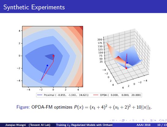
9. Synthetic Experiments: To visualize a comparison, we plot the optimization trajectories on a simple two-dimensional synthetic function in this figure. Our method, OPDA, is noted by the red line, and proximal-gradient descent, is noted by the blue line, as the baseline. After the same number of iterations, we see that our method converges to the minimum with a faster speed.

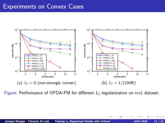
10. Experiments on Convex Cases: We also do some experiments on logistic regression with both L_2 and L_1 regularizations for binary classification. In this part, we compare our method with the proximal-SVRG method, which is also linearly-convergent. In the figure, Y-axis notes the suboptimality, which means how far is the current objective function to the minimum value, and X-axis represents the number of data passes. We found a stable result that OPDA runs faster than proximal-SVRG with different step sizes, L2 regularization, and L1 regularization.

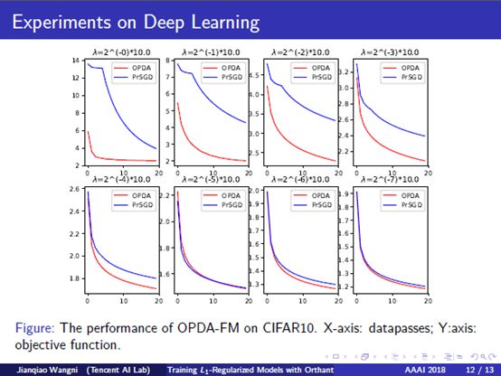
11. Experiments on Deep Learning: We also conducted experiments with L-1 regularized convolutional neural networks, or sparse CNN, to demonstrate the efficiency under the nonconvex case. This application is also useful to reduce the parameter size of neural networks. The red line represents our method, and the blue line is the proximal-SVRG. We test different scales of L1-regularization. We see that OPDA converge faster than proximal-SVRG, and the difference is stronger if the L1 regularization is stronger. Actually, by the orthant-wise nature of our methods, lots of dimensions of the descent direction and the updated points are forced to sparse during alignment, making the equivalent speed much slower, however, our methods still converge much faster than the proximal methods, with the same step size. This proves that our propose dalignment operator does calibrate the direction to be better, making the overall framework more efficient in terms of iterations, but with only negligible extra arithmetic operations.