转录组上游分析，Count计算

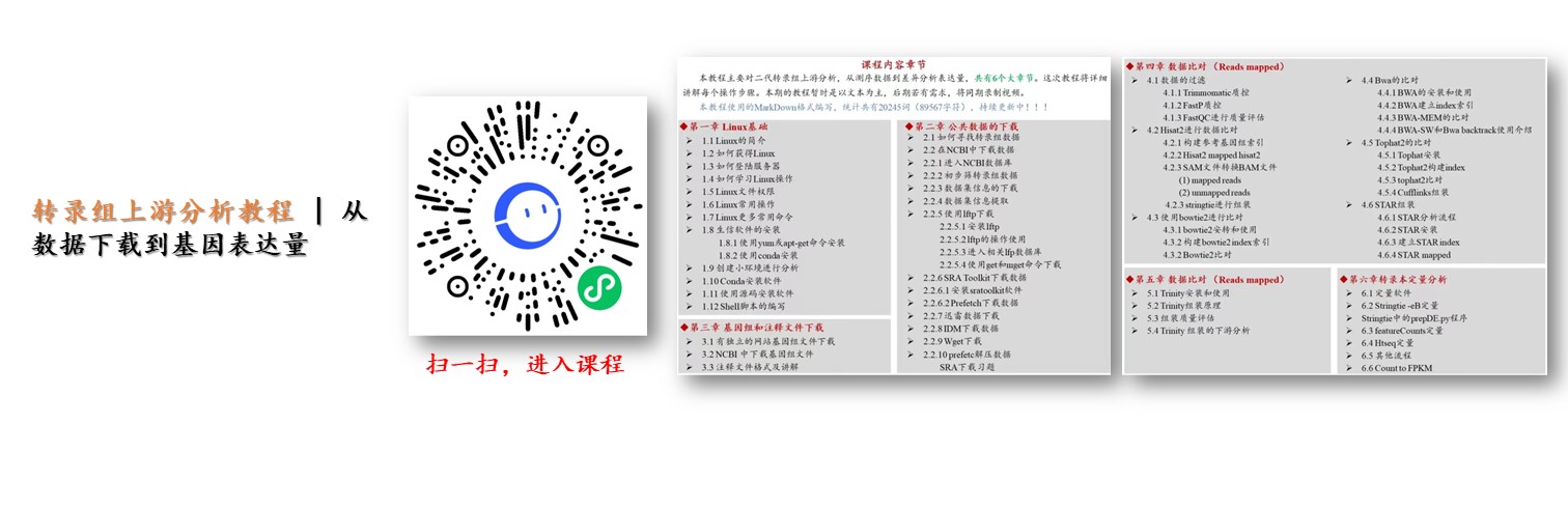
本文主要是介绍转录组上游分析，Count计算，希望对大家解决编程问题提供一定的参考价值，需要的开发者们随着小编来一起学习吧！

本期教程原文链接：转录组定量，最简单的操作，你会吗？

本期教程

第六章 转录本定量分析

定量软件有RSEM,eXpress,salmoe,kallisto，featureCounts。在网络中吗，都有比较详细的教程，大家可以自己去学习。

本教程中推荐使用两种方式获得转录本的表达量，stringtie -eB，featureCounts,stringtie自带的脚本程序prepDE.py。

6.1 Stringtie -eB

Stringtie -eB是通过stringtie组装后的merge.gtf注释信息二次与.bam文件进行转录本表达量的比对，获得转录本的FPKM，此后使用Ballgown 包结合使用，进行后续的分析。详情可看Transcript-level expression analysis of RNA-seq experiments with HISAT, StringTie and Ballgown, 2016, Nat Protoc一文。

此步骤操作后，每个样本会获得新的gtf文件。

stringtie –e –B -p 8 -G stringtie_merged.gtf -o ballgown/ERR188245/ERR188245_chrX.gtf ERR188245_chrX.bam

使用R语言中的ballgown进行分析

pheno_data = read.csv("geuvadis_phenodata.csv")
bg_chrX = ballgown(dataDir = "ballgown", samplePattern = "ERR", pData=pheno_data)
bg_chrX_filt = subset(bg_chrX,"rowVars(texpr(bg_chrX)) >1",genomesubset=TRUE)
results_transcripts = stattest(bg_chrX_filt, feature="transcript",covariate="sex",adjustvars = c("population"), getFC=TRUE, meas="FPKM")
##
# Identify genes that show statistically significant differences between groups. For this we can run the same  function that we used to identify differentially expressed transcripts, but here we set feature="gene" in the stattest command:
results_genes = stattest(bg_chrX_filt, feature="gene", covariate="sex", adjustvars = c("population"), getFC=TRUE, meas="FPKM")#  Add gene names and gene IDs to the results_transcripts data frame:
results_transcripts = data.frame(geneNames=ballgown::geneNames(bg_chrX_filt), geneIDs=ballgown::geneIDs(bg_chrX_filt), results_transcripts)#Sort the results from the smallest P value to the largest:
results_transcripts = arrange(results_transcripts,pval)
results_genes = arrange(results_genes,pval)

# Write the results to a csv file that can be shared and distributed:
write.csv(results_transcripts, "chrX_transcript_results.csv", row.names=FALSE)
write.csv(results_genes, "chrX_gene_results.csv", row.names=FALSE) 
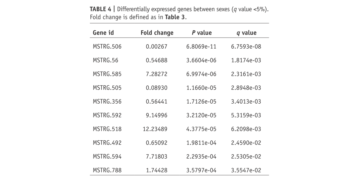
# Identify transcripts and genes with a q value <0.05:
subset(results_transcripts,results_transcripts$qval<0.05)
subset(results_genes,results_genes$qval<0.05)

# Make the plots pretty. This step is optional, but if you do run it you will get the plots in the nice colors that we used to generate our figures:tropical= c('darkorange', 'dodgerblue', 'hotpink', 'limegreen', 'yellow')
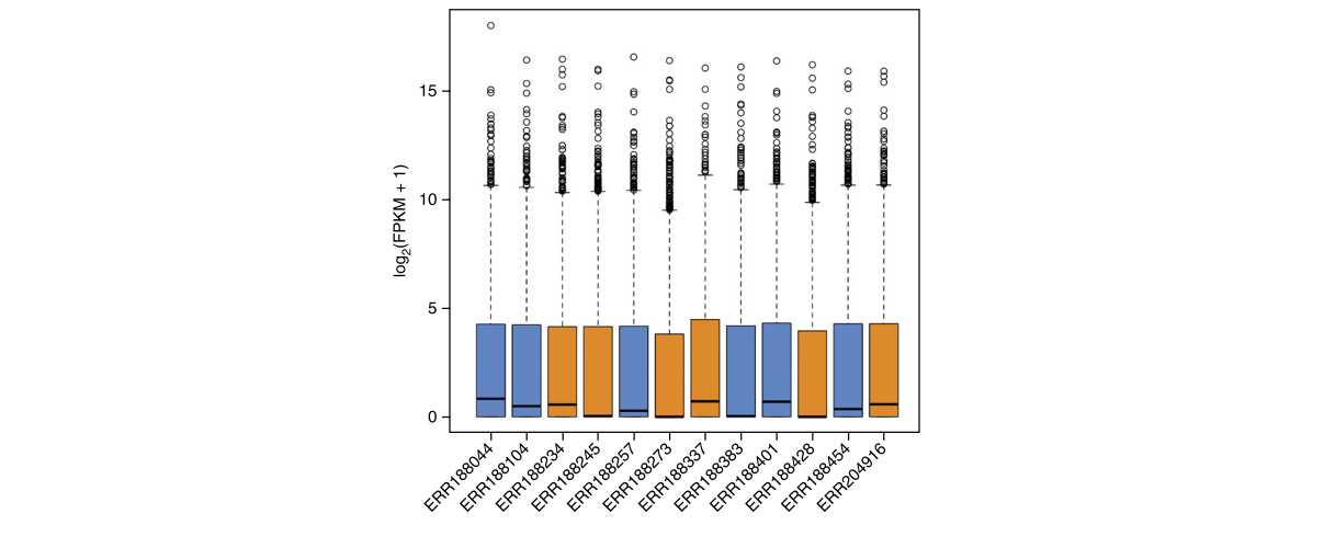
palette(tropical)##  Show the distribution of gene abundances (measured as FPKM values) across samples, colored by sex (Fig. 3).  
fpkm = texpr(bg_chrX,meas="FPKM")
fpkm = log2(fpkm+1)
boxplot(fpkm,col=as.numeric(pheno_data$sex),las=2,ylab='log2(FPKM+1)')

# Make plots of individual transcripts across samples. For example, here we show how to create a plot for the 12th transcript in the data set (Fig. 4). The first two commands below show the name of the transcript (NM_012227) and the name of the gene that contains it (GTP binding protein 6, GTPBP6):
ballgown::transcriptNames(bg_chrX)[12]
##      12 
## "NM_012227"
ballgown::geneNames(bg_chrX)[12]
##      12 
## "GTPBP6"
plot(fpkm[12,] ~ pheno_data$sex, border=c(1,2), main=paste(ballgown::geneNames(bg_chrX)[12],' :', ballgown::transcriptNames(bg_chrX)[12]),pch=19, xlab="Sex", ylab='log2(FPKM+1)')
points(fpkm[12,] ~ jitter(as.numeric(pheno_data$sex)), col=as.numeric(pheno_data$sex))

6.2 Stringtie中的prepDE.py程序

prepDE.py是stringtie软件中自带的获得转录本丰度的脚本，6.1中的HISAT2+Stringtie+Ballgown是一组黄金组合，但是还有很多的局限性。因此，个人建议仍是获得count值，后再进一步的分析，这样的方法更利于下游分析。

具体详情可查看官方文档：http://ccb.jhu.edu/software/stringtie/index.shtml?t=manual

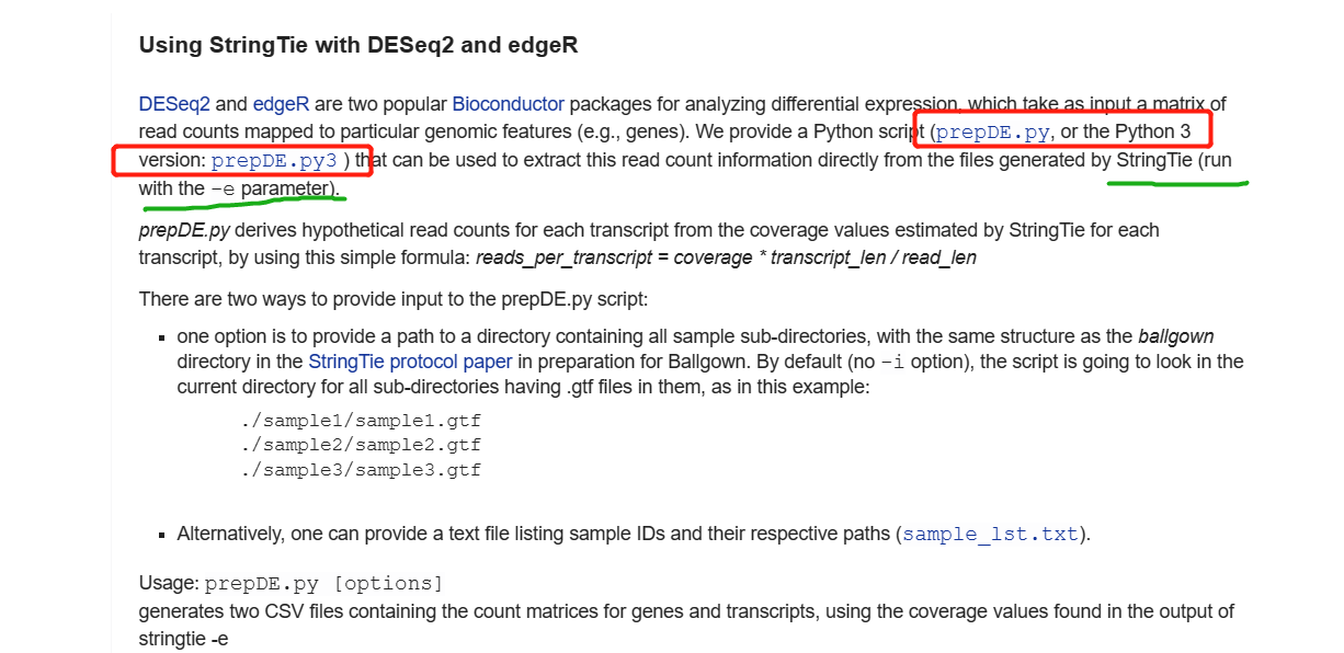
注意：

1. prepDE.py脚本需要输入strintie -e输出的gtf文件
2. 此外，需要获得gtf文件的路径，sample_lst.txt

本期教程原文链接：转录组定量，最简单的操作，你会吗？

prepDE.py -h
Usage: prepDE.py [options]Generates two CSV files containing the count matrices for genes and
transcripts, using the coverage values found in the output of `stringtie -e`Options:-h, --help            show this help message and exit-i INPUT, --input=INPUT, --in=INPUTa folder containing all sample sub-directories, or atext file with sample ID and path to its GTF file oneach line [default: ./]-g G                  where to output the gene count matrix [default:gene_count_matrix.csv-t T                  where to output the transcript count matrix [default:transcript_count_matrix.csv]-l LENGTH, --length=LENGTHthe average read length [default: 75]-p PATTERN, --pattern=PATTERNa regular expression that selects the samplesubdirectories-c, --cluster         whether to cluster genes that overlap with differentgene IDs, ignoring ones with geneID pattern (seebelow)-s STRING, --string=STRINGif a different prefix is used for geneIDs assigned byStringTie [default: MSTRG]-k KEY, --key=KEY     if clustering, what prefix to use for geneIDs assignedby this script [default: prepG]-v                    enable verbose processing--legend=LEGEND       if clustering, where to output the legend file mappingtranscripts to assigned geneIDs [default: legend.csv]

python prepDE.py -i sample_lst.txt
## 或服务器中的Python版本是Python2或python3
prepDE.py -i sample_lst.txt
#or
prepDE.py3 -i sample_lst.txt

04_Result/Stringtie_eB/SRR6929571/SRR6929571.gtf
04_Result/Stringtie_eB/SRR6929572/SRR6929572.gtf
04_Result/Stringtie_eB/SRR6929573/SRR6929573.gtf
04_Result/Stringtie_eB/SRR6929574/SRR6929574.gtf
04_Result/Stringtie_eB/SRR6929577/SRR6929577.gtf
04_Result/Stringtie_eB/SRR6929578/SRR6929578.gtf

gene_count_matrix.csv
transcript_count_matrix.csv

## gene_count_matrix.csv
gene_id,SRR6929571,SRR6929572,SRR6929573,SRR6929574,SRR6929577,SRR6929578
gene:Solyc02g160570.1,0,0,0,0,0,0
gene:Solyc02g161280.1,0,0,0,0,0,0
gene:Solyc01g017370.2,0,0,0,0,0,0
MSTRG.28366,3998,4147,4277,3955,4164,2001## transcript_count_matrix.csv
transcript_id,SRR6929571,SRR6929572,SRR6929573,SRR6929574,SRR6929577,SRR6929578
mRNA:Solyc06g071220.1.1,19,26,41,62,110,33
mRNA:Solyc07g161730.1.1,0,0,0,0,0,0
MSTRG.23978.1,3,0,0,0,0,0
mRNA:Solyc06g062940.5.1,27523,17069,18415,14892,15523,36301
MSTRG.28358.2,13,18,57,32,6,9
mRNA:Solyc05g055535.1.1,0,0,0,0,0,0
MSTRG.28358.1,123,20,410,192,52,134

sed 's/,/\t/g' gene_count_matrix.csv > 01.gene_count.csv

本期教程原文链接：转录组定量，最简单的操作，你会吗？

6.3 featureCounts的使用

featureCounts是subread中脚本，可以使用subread流程进行定量，在这里直接使用前面mapped的bam文件进行转录本定量。

安装：

conda安装

conda install -y subread

源码安装：

官网:[https://sourceforge.net/projects/subread/

wget https://sourceforge.net/projects/subread/files/subread-2.0.3/subread-2.0.3-Linux-x86_64.tar.gz
tar -zxvf subread-2.0.3-Linux-x86_64.tar.gz
cd subread-2.0.3-Linux-x86_64
cd bin/
#
echo 'PATH=$PATH:~/software/subread-2.0.3-Linux-x86_64/bin' >> ~/.bachrc

运行：

使用featureCounts进行定量的bam文件，我建议使用前期使用hisat2。bowtie2，bwa，或是STAR等mapped的文件。

• featureCounts可以对转录本（trancript_id）进行定量
• featureCounts也可以对基因(gene_id)进行定量

Usage: featureCounts [options] -a <annotation_file> -o <output_file> input_file1 [input_file2] ... 

–

featureCounts -T 5 -p -t exon -g transcript_id -a annotation.gtf -o  counts.txt   *.bam

参数：

-T 运行线程数
-t 设置feature-type,在GTF注释中指定特征类型。如果提供多个类型，它们之间应以','隔开，中间没有空格。默认情况下是 "exon"
-g GTF注释文件需要计算的基因或转录本的表达水平。默认是：gene_id，可选择transcript_id
-a提供的注释文件，可以是参考基因组的annotation.gtf，也可以是组转后的gtf文件
-J对可变剪切进行计数
-G < string >当-J设置的时候，通过-G提供一个比对的时候使用的参考基因组文件，辅助寻找可变剪切
-o < string >输出文件的名字，输出文件的内容为read 的统计数目
-O允许多重比对，即当一个read比对到多个feature或多个metafeature的时候，这条read会被统计多次
-d < int >最短的fragment，默认是50
-D < int >最长的fragmen，默认是600-p能用在paired-end的情况中，会统计fragment而不统计read
-B在-p选择的条件下，只有两端read都比对上的fragment才会被统计
-C在-p选择的条件下，只有两端read都比对上的fragment才会被统计

运行：

featureCounts -T 20 -p -t exon -g transcript_id -a stringtie_merged.gtf -o All.transcript.count.txt *.sort.bam

获得结果：

All.transcript.count.txt
All.transcript.count.txt.summary

本期教程原文链接：转录组定量，最简单的操作，你会吗？

6.4 Htseq定量

HTseq-count也是一个比较常用的软件，与featureCount功能一样用来计数（count)

安装：

conda install -y htseq

htseq-count -f bam -r name -s no -a 10 -t exon -i gene_id -m intersection-nonempty yourfile_name.bam ~/reference/hisat2_reference/Homo_sapiens.GRCh38.86.chr_patch_hapl_scaff.gtf > counts.txt

usage: htseq-count [options] alignment_file gff_file-f {sam,bam}  (default: sam)#设置输入文件的格式，该参数的值可以是sam或bam。
-r {pos,name}  (default: name)#设置sam或bam文件的排序方式，该参数的值可以是name或pos。#前者表示按read名进行排序，后者表示按比对的参考基因组位置进行排序。#若测序数据是双末端测序，当输入sam/bam文件是按pos方式排序的时候，#两端reads的比对结果在sam/bam文件中一般不是紧邻的两行，#程序会将reads对的第一个比对结果放入内存，直到读取到另一端read的比对结果。#因此，选择pos可能会导致程序使用较多的内存，它也适合于未排序的sam/bam文件。#而pos排序则表示程序认为双末端测序的reads比对结果在紧邻的两行上，#也适合于单端测序的比对结果。很多其它表达量分析软件要求输入的sam/bam文件是按pos排序的，但HTSeq推荐使用name排序，且一般比对软件的默认输出结果也是按name进行排序的。
-s {yes,no,reverse}  (default: yes) #数据是否来源于链特异性测序，链特异性是指在建库测序时，只测mRNA反转录出的cDNA序列，而不测该cDNA序列反向互补的另一条DNA序列；换句话说就是，链特异性能更准确反映出mRNA的序列信息
-a MINAQUAL (default: 10)#忽略比对质量低于此值的比对结果
-t FEATURETYPE #feature type (3rd column in GFF file) to be used, all features of other type are ignored (default, suitable for Ensembl GTF files: exon)#程序会对该指定的feature（gtf/gff文件第三列）进行表达量计算，而gtf/gff文件中其它的feature都会被忽略。
-i IDATTR#GFF attribute to be used as feature ID (default, suitable for Ensembl GTF files: gene_id)#设置feature ID是由gtf/gff文件第9列那个标签决定的；若gtf/gff文件多行具有相同的feature ID，则它们来自同一个feature，程序会计算这些features的表达量之和赋给相应的feature ID。
-m {union,intersection-strict,intersection-nonempty} (default: union)#设置表达量计算模式。该参数的值可以有union, intersection-strict and intersection-nonempty。这三种模式的选择请见上面对这3种模式的示意图。从图中可知，对于原核生物，推荐使用intersection-strict模式；对于真核生物，推荐使用union模式。
-o | --samout#输出一个sam文件，该sam文件的比对结果中多了一个XF标签，表示该read比对到了某个feature上。
-n #指定多线程，默认是1

运行Htseq-count：

htseq-count -f bam -r name -s no -a 10 -t exon -i transcript_id -m intersection-strict ../../03_MappedFile/Hisat2_Mapped/*.bam ../../02_Geneome_index/ITAG4.1_gene_models.gtf > htseq_counts.txt

6.5 其他流程

salmon 流程

软件官网：https://combine-lab.github.io/salmon/

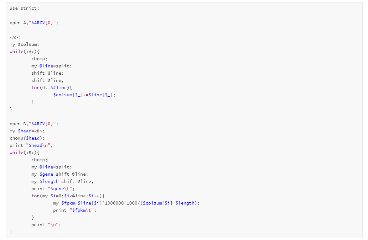
6.6 Count to FPKM

• count to FPKM

使用Perl脚本进行转换

## 需要信息
1. 基因名
2. 基因长度
3. count值

使用cut提取信息：

cat All.transcript.count.txt | cut -f 1,6-13 > 01.all.count.txt

运行perl脚本：

perl CountToFPKM.pl 01.all.count.txt > 02.all.FPKM.txt

CountToFPKM.pl脚本：

本期教程原文链接：转录组定量，最简单的操作，你会吗？

往期教程部分内容

往期部分文章

1. 复现SCI文章系列专栏

2. 《生信知识库订阅须知》,同步更新，易于搜索与管理。

3. 最全WGCNA教程（替换数据即可出全部结果与图形）

• WGCNA分析 | 全流程分析代码 | 代码一

• WGCNA分析 | 全流程分析代码 | 代码二

• WGCNA分析 | 全流程代码分享 | 代码三

• WGCNA分析 | 全流程分析代码 | 代码四

• WGCNA分析 | 全流程分析代码 | 代码五(最新版本)

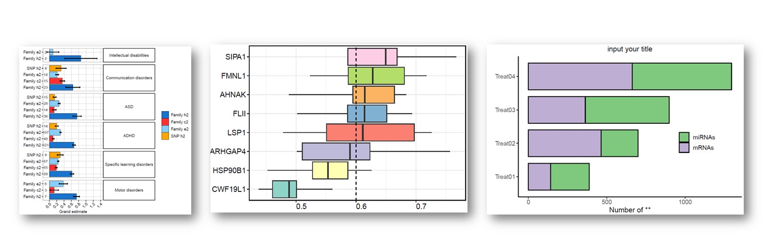
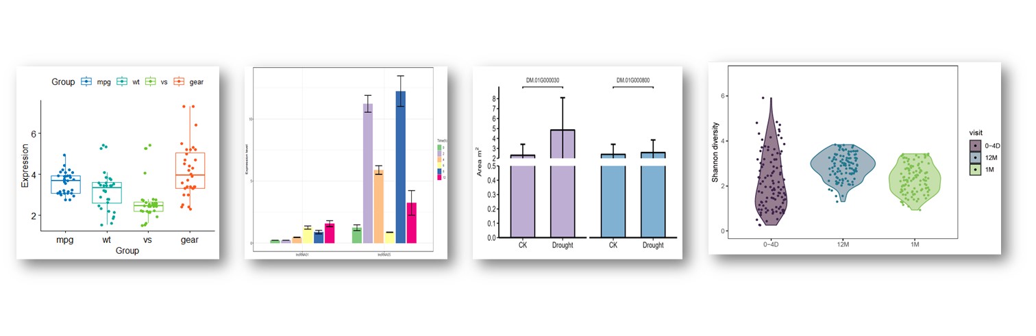
4. 精美图形绘制教程

• 精美图形绘制教程

5. 转录组分析教程

• 转录组上游分析教程[零基础]

• 一个转录组上游分析流程 | Hisat2-Stringtie

6. 转录组下游分析

• 批量做差异分析及图形绘制 | 基于DESeq2差异分析

• GO和KEGG富集分析

• 单基因GSEA富集分析

• 全基因集GSEA富集分析

小杜的生信筆記 ，主要发表或收录生物信息学的教程，以及基于R的分析和可视化（包括数据分析，图形绘制等）；分享感兴趣的文献和学习资料!!

这篇关于转录组上游分析，Count计算的文章就介绍到这儿，希望我们推荐的文章对编程师们有所帮助！