Tensorflow2.0学习（2）：基于fashion_mnist数据集的分类基本步骤

本文主要是介绍Tensorflow2.0学习（2）：基于fashion_mnist数据集的分类基本步骤，希望对大家解决编程问题提供一定的参考价值，需要的开发者们随着小编来一起学习吧！

导入包、打印包的信息

其中 %matplotlib inline 是IPython中的魔法函数，作用是：在利用matplotlib.pyplot作图或创建画布时不需要plt.show()，即可实现图像的显示。

import matplotlib as mpl
import matplotlib.pyplot as plt
%matplotlib inline
import numpy as np
import sklearn
import pandas as pd
import os
import sys
import time
import tensorflow as tf
from tensorflow import keras
print(tf.__version__)
print(sys.version_info)
for module in mpl, np ,pd, sklearn, tf, keras:print(module.__name__, module.__version__)

2.1.0
sys.version_info(major=3, minor=7, micro=4, releaselevel='final', serial=0)
matplotlib 3.1.1
numpy 1.16.5
pandas 0.25.1
sklearn 0.21.3
tensorflow 2.1.0
tensorflow_core.python.keras.api._v2.keras 2.2.4-tf

下载、读取、分割数据集

# 读取keras中的进阶版mnist数据集
fashion_mnist = keras.datasets.fashion_mnist
# 加载数据集，切分为训练集和测试集
(x_train_all, y_train_all), (x_test, y_test) = fashion_mnist.load_data()
# 从训练集中将后五千张作为验证集，前五千张作为训练集
# [:5000]默认从头开始，从头开始取5000个
# [5000:]从第5001开始，结束位置默认为最后
x_valid, x_train = x_train_all[:5000], x_train_all[5000:]
y_valid, y_train = y_train_all[:5000], y_train_all[5000:]
# 打印这些数据集的大小
print(x_valid.shape, y_valid.shape)
print(x_train.shape, y_train.shape)
print(x_test.shape, y_test.shape)

Downloading data from https://storage.googleapis.com/tensorflow/tf-keras-datasets/train-images-idx3-ubyte.gz
26427392/26421880 [==============================] - 7s 0us/step
Downloading data from https://storage.googleapis.com/tensorflow/tf-keras-datasets/t10k-labels-idx1-ubyte.gz
8192/5148 [===============================================] - 0s 0us/step
Downloading data from https://storage.googleapis.com/tensorflow/tf-keras-datasets/t10k-images-idx3-ubyte.gz
4423680/4422102 [==============================] - 1s 0us/step
(5000, 28, 28) (5000,)
(55000, 28, 28) (55000,)
(10000, 28, 28) (10000,)

可以得出，训练集有55000张图片，每张图片为28*28；验证集有5000张图片；测试集有1000张图片。

显示图片

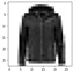
def show_single_image(img_arr):plt.imshow(img_arr, cmap="binary")plt.show()
# 显示训练集第一张图片    
show_single_image(x_train[0])

在这里插入图片描述

# 设置n_rows行与n_cols列用来显示图像，共显示x_data个图像
#（y_data是其标签，class_names是其真实的类名）
def show_imgs(n_rows, n_cols, x_data, y_data, class_names):# 断言：不满足条件触发异常assert len(x_data) == len(y_data)assert n_rows * n_cols <len(x_data)plt.figure(figsize=(n_cols * 1.4, n_rows * 1.6))for row in range(n_rows):for col in range(n_cols):index = n_cols * row + col# 总的图像为n_rows * n_cols,当前图像位置为index+1plt.subplot(n_rows, n_cols, index+1)plt.imshow(x_data[index], cmap="binary",interpolation = 'nearest')plt.axis('off')plt.title(class_names[y_data[index]])plt.show()
class_names = ['T-shirt','Trouser','Pullover','Dress','Coat', 'Sandal', 'Shirt', 'Sneaker', 'Bag','Ankle boot']
# 显示训练集的十五张图片              
show_imgs(3, 5, x_train, y_train, class_names)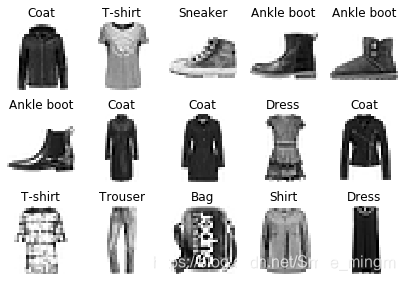

在这里插入图片描述

构建模型

# tf.keras.models.Sequential() 构建模型的容器# 创建一个Sequential的对象,顺序模型，多个网络层的线性堆叠
# 可使用add方法将各层添加到模块中
model = keras.models.Sequential()# 添加层次
# 输入层：Flatten将28*28的图像矩阵展平成为一个一维向量
model.add(keras.layers.Flatten(input_shape=[28,28]))# 全连接层（上层所有单元与下层所有单元都连接）：
# 第一层300个单元，第二层100个单元，激活函数为 relu:
# relu: y = max(0, x)
model.add(keras.layers.Dense(300,activation="relu"))          
model.add(keras.layers.Dense(100,activation="relu"))# 输出为长度为10的向量，激活函数为 softmax:
# softmax: 将向量变成概率分布，x = [x1, x2, x3],
# y = [e^x1/sum, e^x2/sum, e^x3/sum],sum = e^x1+e^x2+e^x3
model.add(keras.layers.Dense(10,activation="softmax"))# 目标函数的构建与求解方法
# 为什么使用sparse? : 
# y->是一个数，要用sparse_categorical_crossentropy
# y->是一个向量，直接用categorical_crossentropy
model.compile(loss="sparse_categorical_crossentropy",optimizer="adam",metrics = ["accuracy"])
"""
构建模型也可以这样：
model = keras.models.Sequential([keras.layers.Flatten(input_shape=[28,28]),keras.layers.Dense(300,activation="relu"),keras.layers.Dense(300,activation="relu"),keras.layers.Dense(10,activation="softmax")
])"""

查看模型

# 看模型的层情况
model.layers

[<tensorflow.python.keras.layers.core.Flatten at 0x28a9c583088>,<tensorflow.python.keras.layers.core.Dense at 0x28a9c583108>,<tensorflow.python.keras.layers.core.Dense at 0x28a9c5cbec8>,<tensorflow.python.keras.layers.core.Dense at 0x28a9c925f88>]

# 看模型的概况
model.summary()# 参数量：[None,784] * w + b -> [None, 300]:w.shape=[784, 300],b = 300

Model: "sequential"
_________________________________________________________________
Layer (type)                 Output Shape              Param #   
=================================================================
flatten (Flatten)            (None, 784)               0         
_________________________________________________________________
dense (Dense)                (None, 300)               235500    
_________________________________________________________________
dense_1 (Dense)              (None, 100)               30100     
_________________________________________________________________
dense_2 (Dense)              (None, 10)                1010      
=================================================================
Total params: 266,610
Trainable params: 266,610
Non-trainable params: 0
_________________________________________________________________

训练

# 开启训练
# epochs:训练集遍历10次
# validation_data:每个epoch就会用验证集验证
# 会发现loss和accuracy到后面一直不变，因为用sgd梯度下降法会导致陷入局部最小值点
# 因此将loss函数的下降方法改为 adam
history = model.fit(x_train, y_train, epochs=10,validation_data=(x_valid, y_valid))

Train on 55000 samples, validate on 5000 samples
Epoch 1/10
55000/55000 [==============================] - 4s 69us/sample - loss: 2.5882 - accuracy: 0.7635 - val_loss: 0.6161 - val_accuracy: 0.8122
Epoch 2/10
55000/55000 [==============================] - 3s 62us/sample - loss: 0.5384 - accuracy: 0.8169 - val_loss: 0.5430 - val_accuracy: 0.8268
Epoch 3/10
55000/55000 [==============================] - 3s 62us/sample - loss: 0.4813 - accuracy: 0.8317 - val_loss: 0.5800 - val_accuracy: 0.8166
Epoch 4/10
55000/55000 [==============================] - 3s 63us/sample - loss: 0.4575 - accuracy: 0.8381 - val_loss: 0.5061 - val_accuracy: 0.8276
Epoch 5/10
55000/55000 [==============================] - 3s 62us/sample - loss: 0.4363 - accuracy: 0.8447 - val_loss: 0.4295 - val_accuracy: 0.8612
Epoch 6/10
55000/55000 [==============================] - 3s 62us/sample - loss: 0.4133 - accuracy: 0.8530 - val_loss: 0.4093 - val_accuracy: 0.8602
Epoch 7/10
55000/55000 [==============================] - 3s 63us/sample - loss: 0.3913 - accuracy: 0.8603 - val_loss: 0.4328 - val_accuracy: 0.8506
Epoch 8/10
55000/55000 [==============================] - 3s 63us/sample - loss: 0.3798 - accuracy: 0.8635 - val_loss: 0.3907 - val_accuracy: 0.8564
Epoch 9/10
55000/55000 [==============================] - 4s 64us/sample - loss: 0.3694 - accuracy: 0.8681 - val_loss: 0.4227 - val_accuracy: 0.8564
Epoch 10/10
55000/55000 [==============================] - 4s 64us/sample - loss: 0.3625 - accuracy: 0.8696 - val_loss: 0.4136 - val_accuracy: 0.8630

查看训练后的结果

type(history)

tensorflow.python.keras.callbacks.History

history.history
# loss是训练集的损失值，val_loss是测试集的损失值

{'loss': [2.5882461955070495,0.5384013248010115,0.48129710446704516,0.45748968857851896,0.43628633408329703,0.41328840144330803,0.3912581247546456,0.37976206094351683,0.3693601242488081,0.3625139371091669],'accuracy': [0.7634909,0.81685454,0.8316727,0.83805454,0.84467274,0.8529818,0.8602909,0.8634727,0.86814547,0.8695818],'val_loss': [0.6161495039701462,0.542988519859314,0.5799951359272003,0.506083318400383,0.4295428094863892,0.40931380726099015,0.4327934848666191,0.39065408419966696,0.42266337755918504,0.41358628759980204],'val_accuracy': [0.8122,0.8268,0.8166,0.8276,0.8612,0.8602,0.8506,0.8564,0.8564,0.863]}

def plot_learning_curves(history):# 将history.history转换为dataframe格式pd.DataFrame(history.history).plot(figsize=(8, 5 ))plt.grid(True)# gca：get current axes,gcf: get current figureplt.gca().set_ylim(0, 1)plt.show()
plot_learning_curves(history)

[外链图片转存失败,源站可能有防盗链机制,建议将图片保存下来直接上传(img-PzEQNq8y-1582528839439)(output_10_0.png)]

# 转换为dataframe格式进行查看
pd.DataFrame(history.history)

	loss	accuracy	val_loss	val_accuracy
0	2.588246	0.763491	0.616150	0.8122
1	0.538401	0.816855	0.542989	0.8268
2	0.481297	0.831673	0.579995	0.8166
3	0.457490	0.838055	0.506083	0.8276
4	0.436286	0.844673	0.429543	0.8612
5	0.413288	0.852982	0.409314	0.8602
6	0.391258	0.860291	0.432793	0.8506
7	0.379762	0.863473	0.390654	0.8564
8	0.369360	0.868145	0.422663	0.8564
9	0.362514	0.869582	0.413586	0.8630