本文主要是介绍立体匹配算法(Stereo correspondence),希望对大家解决编程问题提供一定的参考价值,需要的开发者们随着小编来一起学习吧!
SGM(Semi-Global Matching)原理:
SGM的原理在wiki百科和matlab官网上有比较详细的解释:
wiki matlab
如果想完全了解原理还是建议看原论文 paper(我就不看了,懒癌犯了。)
优质论文解读和代码实现
一位大神自己用c++实现的SGM算法github
先介绍两个重要的参数:
注:这一部分参考的是matlab的解释,后面的部分是参考的opencv的实现,细节可能有些出入,大体上是一致的。
Disparity Levels and Number of Directions
Disparity Levels
Disparity Levels: Disparity levels is a parameter used to define the search space for matching. As shown in figure below, the algorithm searches for each pixel in the Left Image from among D pixels in the Right Image. The D values generated are D disparity levels for a pixel in Left Image. The first D columns of Left Image are unused because the corresponding pixels in Right Image are not available for comparison. In the figure, w represents the width of the image and h is the height of the image. For a given image resolution, increasing the disparity level reduces the minimum distance to detect depth. Increasing the disparity level also increases the computation load of the algorithm. At a given disparity level, increasing the image resolution increases the minimum distance to detect depth. Increasing the image resolution also increases the accuracy of depth estimation. The number of disparity levels are proportional to the input image resolution for detection of objects at the same depth. This example supports disparity levels from 8 to 128 (both values inclusive). The explanation of the algorithm refers to 64 disparity levels. The models provided in this example can accept input images of any resolution.——matlab
字太多,看不懂,让gpt解释了一下:
# gpt生成,仅供本人理解SSD原理
import numpy as npdef compute_disparity(left_img, right_img, block_size=5, num_disparities=64):# 图像尺寸height, width = left_img.shape# 初始化视差图disparity_map = np.zeros_like(left_img)# 遍历每个像素for y in range(height):for x in range(width):# 定义搜索范围min_x = max(0, x - num_disparities // 2)max_x = min(width, x + num_disparities // 2)# 提取左图像块left_block = left_img[y:y+block_size, x:x+block_size]# 初始化最小 SSD 和对应的视差min_ssd = float('inf')best_disparity = 0# 在搜索范围内寻找最佳视差for d in range(min_x, max_x):# 提取右图像块right_block = right_img[y:y+block_size, d:d+block_size]# 计算 SSDssd = np.sum((left_block - right_block)**2)# 更新最小 SSD 和对应的视差if ssd < min_ssd:min_ssd = ssdbest_disparity = abs(x - d)# 将最佳视差保存到视差图中disparity_map[y, x] = best_disparityreturn disparity_map# 示例用法
left_img = np.random.randint(0, 255, size=(100, 100), dtype=np.uint8)
right_img = np.roll(left_img, shift=5, axis=1)  # 创建右图,右移了5个像素disparity_map = compute_disparity(left_img, right_img, block_size=5, num_disparities=64)# 可视化结果(这里简化为将视差图缩放以便可视化)
import matplotlib.pyplot as plt
plt.imshow(disparity_map, cmap='gray')
plt.title('Disparity Map')
plt.show()
这样就明白了,Disparity Levels就是计算视差的范围(视差搜索范围)。
Number of Directions
Number of Directions:
Number of Directions: In the SGBM algorithm, to optimize the cost function, the input image is considered from multiple directions. In general, accuracy of disparity result improves with increase in number of directions. This example analyzes five directions: left-to-right (A1), top-left-to-bottom-right (A2), top-to-bottom (A3), top-right-to-bottom-left (A4), and right-to-left (A5).
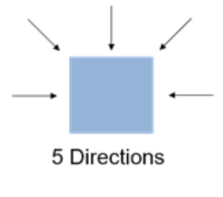
按照单一路径匹配像素不够稳健,按照图像进行二维最优的全局匹配时间复杂度太高(NP完全问题),所以SGM的作者使用一维路径聚合的方式来近似二维最优。

pic 参考
SAD和SSD
用SAD 或者 SSD计算图像相似度,来做匹配。
公式:
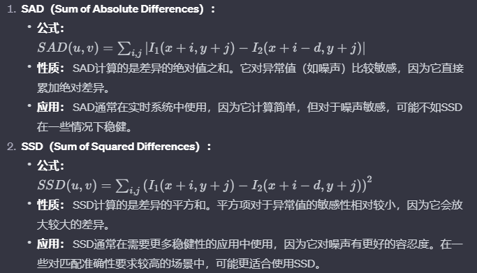
公式和代码虽然是gpt生成的,但是公式看起来没错,代码可以帮助理解,仅供参考。
代码里面的 num_disparities 就是 Disparity Levels
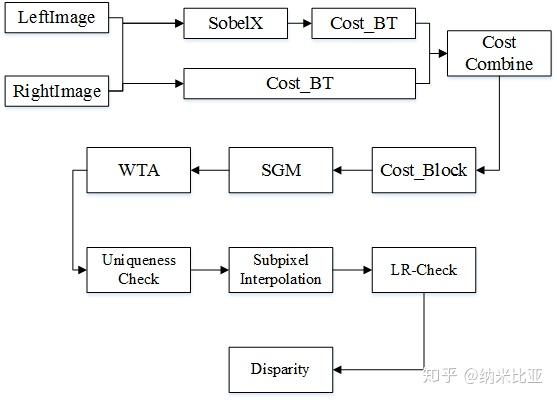
SGBM in opencv
本人用opencv较多,这里仅关注代码在opencv的实现。
opencv StereoSGBM_create示例:
# gpt生成,仅作为参考,具体请查看opencv官方文档https://docs.opencv.org/4.x/d2/d85/classcv_1_1StereoSGBM.html
import cv2
import numpy as np# 读取左右视图
left_image = cv2.imread('left_image.png', cv2.IMREAD_GRAYSCALE)
right_image = cv2.imread('right_image.png', cv2.IMREAD_GRAYSCALE)# 创建SGBM对象
sgbm = cv2.StereoSGBM_create(minDisparity=0,numDisparities=16,  # 视差范围,一般为16的整数倍blockSize=5,        # 匹配块的大小,一般为奇数P1=8 * 3 * 5 ** 2,   # SGBM算法参数P2=32 * 3 * 5 ** 2,  # SGBM算法参数disp12MaxDiff=1,    # 左右视差图的最大差异uniquenessRatio=10,  # 匹配唯一性百分比speckleWindowSize=100,  # 过滤小连通区域的窗口大小speckleRange=32      # 连通区域内的差异阈值
)# 计算视差图
disparity_map = sgbm.compute(left_image, right_image)# 将视差图进行归一化处理
disparity_map = cv2.normalize(disparity_map, None, 0, 255, cv2.NORM_MINMAX)# 显示左图、右图和视差图
cv2.imshow('Left Image', left_image)
cv2.imshow('Right Image', right_image)
cv2.imshow('Disparity Map', disparity_map.astype(np.uint8))cv2.waitKey(0)
cv2.destroyAllWindows()
Difference between SGBM and SGM
what is the difference between opencv sgbm and sgm
opencv官方的解释:
The class implements the modified H. Hirschmuller algorithm [82] that differs from the original one as follows:
- By default, the algorithm is single-pass, which means that you consider only 5 directions instead of 8. Set mode=StereoSGBM::MODE_HH in createStereoSGBM to run the full variant of the algorithm but beware that it may consume a lot of memory.
- The algorithm matches blocks, not individual pixels. Though, setting blockSize=1 reduces the blocks to single pixels.
- Mutual information cost function is not implemented. Instead, a simpler Birchfield-Tomasi sub-pixel metric from [15] is used. Though, the color images are supported as well.
Some pre- and post- processing steps from K. Konolige algorithm StereoBM are included, for example: pre-filtering (StereoBM::PREFILTER_XSOBEL type) and post-filtering (uniqueness check, quadratic interpolation and speckle filtering).
大概的意思就是,与SGM不同之处在于,SGBM算法匹配的时候最小单位是blocks,而不是像素,不过设置blockSize=1的时候,就变成SGM了。没有实现互信息,而是用了更简单的Birchfield-Tomasi sub-pixel metric。除此之外还有一些预处理和后处理操作。
大概是这样,不知道对不对。
深度的立体匹配算法
先开个坑
这篇关于立体匹配算法(Stereo correspondence)的文章就介绍到这儿,希望我们推荐的文章对编程师们有所帮助!


