【小沐学NLP】Python实现K-Means聚类算法（nltk、sklearn）

本文主要是介绍【小沐学NLP】Python实现K-Means聚类算法（nltk、sklearn），希望对大家解决编程问题提供一定的参考价值，需要的开发者们随着小编来一起学习吧！

1、简介

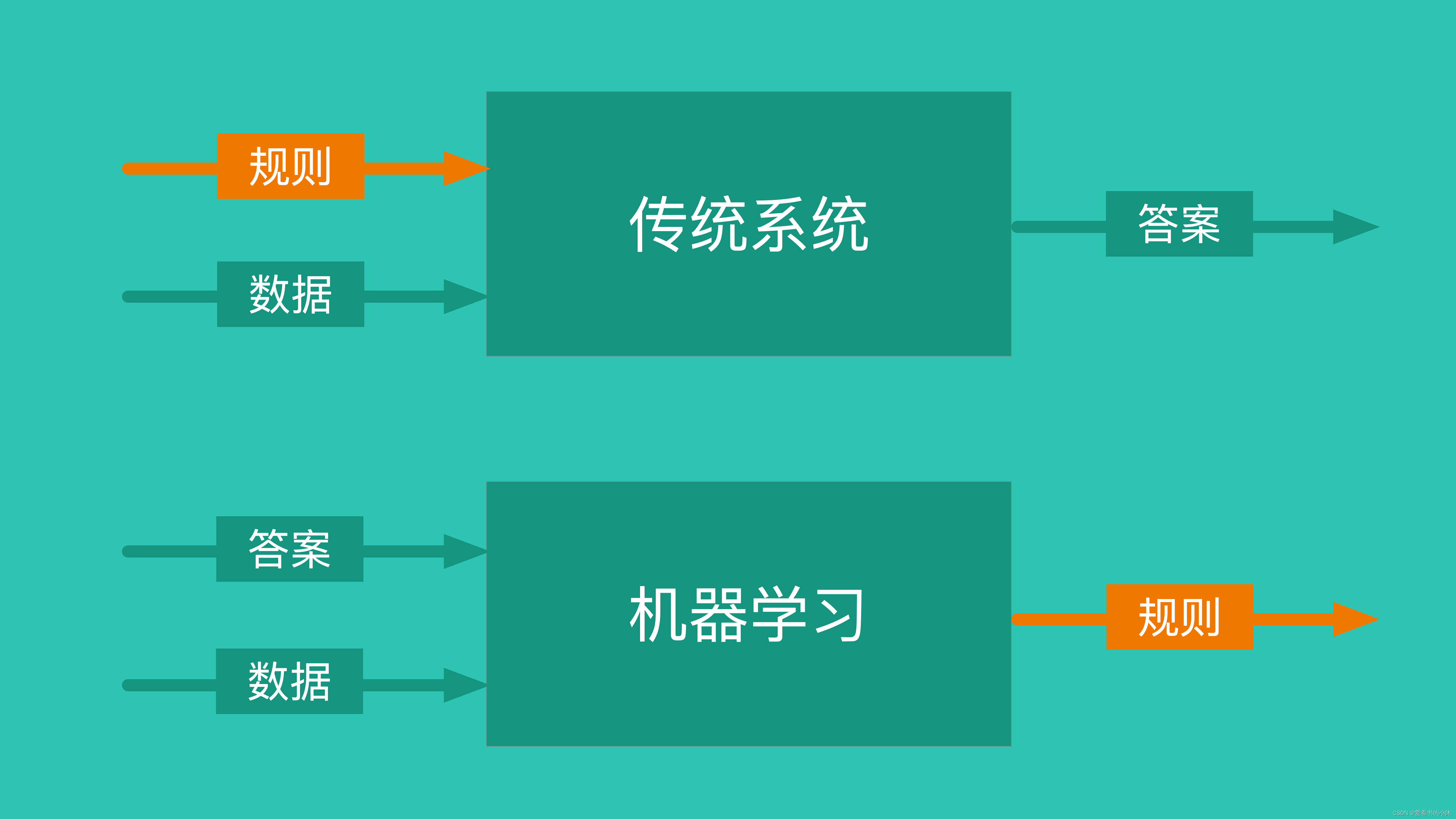
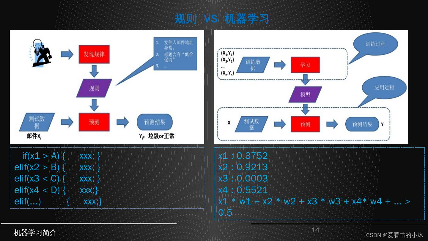
1.1 机器学习

• 机器学习三要素：包括数据、模型、算法
• 机器学习三大任务方向：分类、回归、聚类
• 机器学习三大类训练方法：监督学习、非监督学习、强化学习
  
  
  

1.2 K 均值聚类

1.2.1 聚类定义

聚类是一种无监督学习任务，该算法基于数据的内部结构寻找观察样本的自然族群（即集群）。使用案例包括细分客户、新闻聚类、文章推荐等。
因为聚类是一种无监督学习（即数据没有标注），并且通常使用数据可视化评价结果。如果存在「正确的回答」（即在训练集中存在预标注的集群），那么分类算法可能更加合适。

依据算法原理，聚类算法可以分为基于划分的聚类算法（比如 K-means）、基于密度的聚类算法（比如DBSCAN）、基于层次的聚类算法（比如HC）和基于模型的聚类算法（比如HMM）。

1.2.2 K-Means定义

K 均值聚类是一种通用目的的算法，聚类的度量基于样本点之间的几何距离（即在坐标平面中的距离）。集群是围绕在聚类中心的族群，而集群呈现出类球状并具有相似的大小。聚类算法是我们推荐给初学者的算法，因为该算法不仅十分简单，而且还足够灵活以面对大多数问题都能给出合理的结果。
K-means是基于样本集合划分的聚类算法，是一种无监督学习。

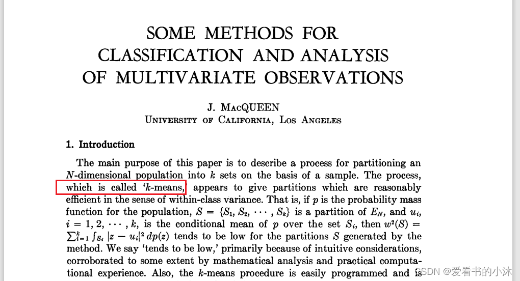
1967年，J. MacQueen 在论文《 Some methods for classification and analysis of multivariate observations》中把这种方法正式命名为 K-means。

https://www.cs.cmu.edu/~bhiksha/courses/mlsp.fall2010/class14/macqueen.pdf

1.2.3 K-Means优缺点

优点：K 均值聚类是最流行的聚类算法，因为该算法足够快速、简单，并且如果你的预处理数据和特征工程十分有效，那么该聚类算法将拥有令人惊叹的灵活性。
缺点：该算法需要指定集群的数量，而 K 值的选择通常都不是那么容易确定的。另外，如果训练数据中的真实集群并不是类球状的，那么 K 均值聚类会得出一些比较差的集群。

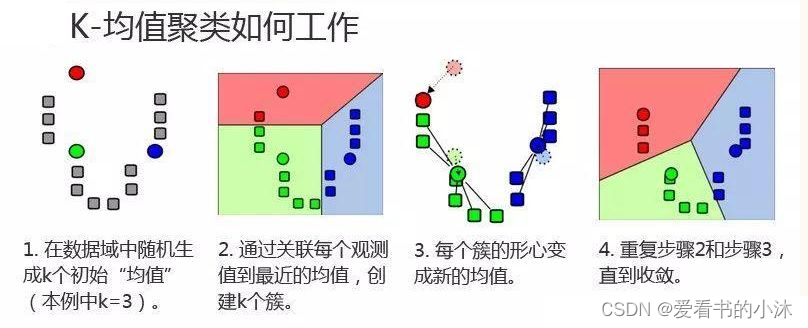
1.2.4 K-Means算法步骤

• 1. 对于给定的一组数据，随机初始化K个聚类中心（簇中心）
• 2. 计算每个数据到簇中心的距离（一般采用欧氏距离），并把该数据归为离它最近的簇。
• 3. 根据得到的簇，重新计算簇中心。
• 4. 对步骤2、步骤3进行迭代直至簇中心不再改变或者小于指定阈值。
     
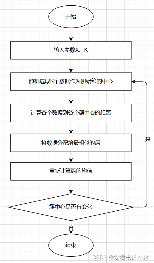
     终止条件可以是：
     没有（或最小数目）对象被重新分配给不同的聚类
     没有（或最小数目）聚类中心再发生变化， 误差 平方和 局部最小。.

K-means聚类算法的主要步骤：
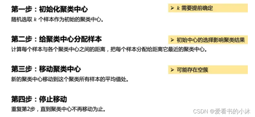
第一步：初始化聚类中心；
第二步：给聚类中心分配样本 ；
第三步：移动聚类中心 ；
第四步：停止移动。
注意：K-means算法采用的是迭代的方法，得到局部最优解.

2、测试

2.1 K-Means（Python）

# -*- coding:utf-8 -*-
import numpy as np
from matplotlib import pyplotclass K_Means(object):# k是分组数；tolerance‘中心点误差’；max_iter是迭代次数def __init__(self, k=2, tolerance=0.0001, max_iter=300):self.k_ = kself.tolerance_ = toleranceself.max_iter_ = max_iterdef fit(self, data):self.centers_ = {}for i in range(self.k_):self.centers_[i] = data[i]for i in range(self.max_iter_):self.clf_ = {}for i in range(self.k_):self.clf_[i] = []# print("质点:",self.centers_)for feature in data:# distances = [np.linalg.norm(feature-self.centers[center]) for center in self.centers]distances = []for center in self.centers_:# 欧拉距离# np.sqrt(np.sum((features-self.centers_[center])**2))distances.append(np.linalg.norm(feature - self.centers_[center]))classification = distances.index(min(distances))self.clf_[classification].append(feature)# print("分组情况:",self.clf_)prev_centers = dict(self.centers_)for c in self.clf_:self.centers_[c] = np.average(self.clf_[c], axis=0)# '中心点'是否在误差范围optimized = Truefor center in self.centers_:org_centers = prev_centers[center]cur_centers = self.centers_[center]if np.sum((cur_centers - org_centers) / org_centers * 100.0) > self.tolerance_:optimized = Falseif optimized:breakdef predict(self, p_data):distances = [np.linalg.norm(p_data - self.centers_[center]) for center in self.centers_]index = distances.index(min(distances))return indexif __name__ == '__main__':x = np.array([[1, 2], [1.5, 1.8], [5, 8], [8, 8], [1, 0.6], [9, 11]])k_means = K_Means(k=2)k_means.fit(x)print(k_means.centers_)for center in k_means.centers_:pyplot.scatter(k_means.centers_[center][0], k_means.centers_[center][1], marker='*', s=150)for cat in k_means.clf_:for point in k_means.clf_[cat]:pyplot.scatter(point[0], point[1], c=('r' if cat == 0 else 'b'))predict = [[2, 1], [6, 9]]for feature in predict:cat = k_means.predict(predict)pyplot.scatter(feature[0], feature[1], c=('r' if cat == 0 else 'b'), marker='x')pyplot.show()

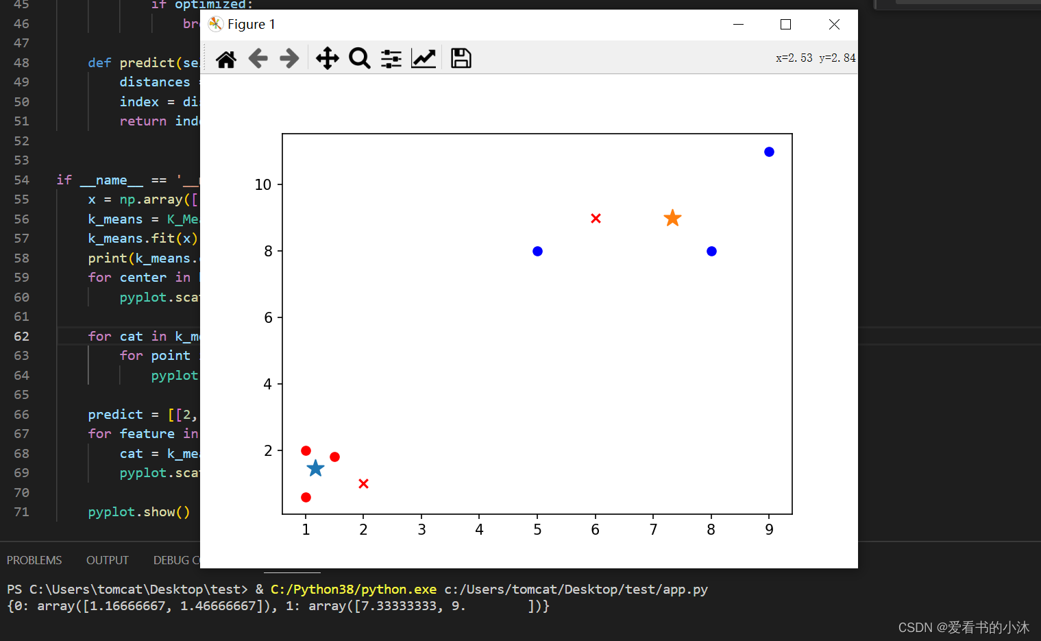
*是两组数据的”中心点”；x是预测点分组。

2.2 K-Means（Sklearn）

http://scikit-learn.org/stable/modules/clustering.html#k-means

2.2.1 例子1：数组分类

# -*- coding:utf-8 -*-
import numpy as np
from matplotlib import pyplot
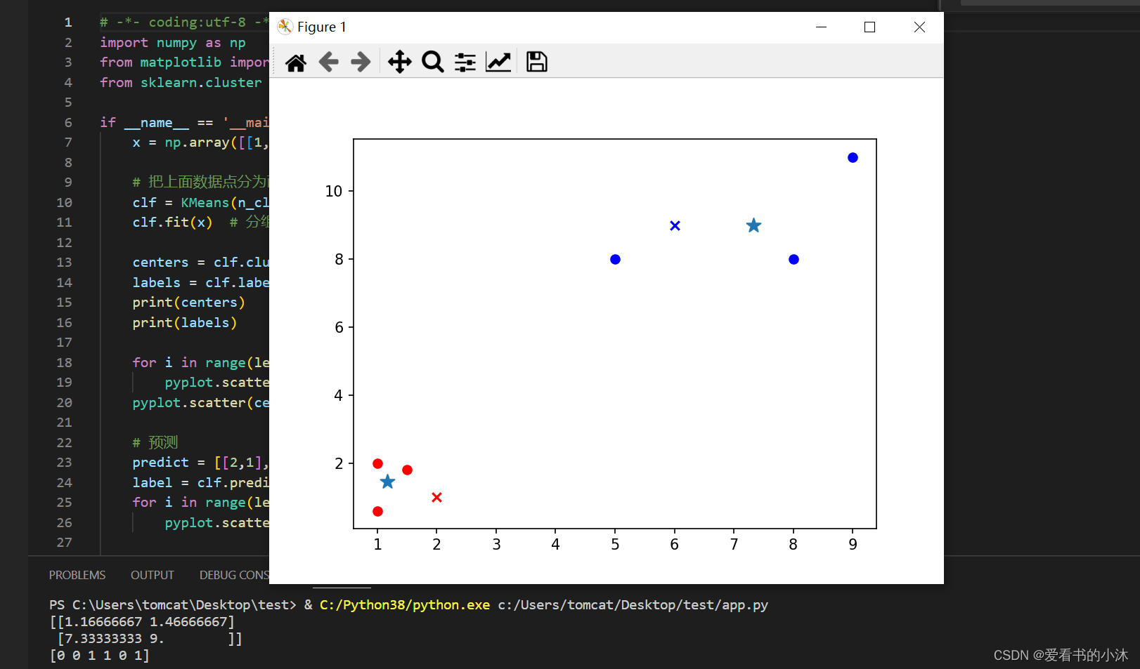
from sklearn.cluster import KMeansif __name__ == '__main__':x = np.array([[1, 2], [1.5, 1.8], [5, 8], [8, 8], [1, 0.6], [9, 11]])# 把上面数据点分为两组（非监督学习）clf = KMeans(n_clusters=2)clf.fit(x)  # 分组centers = clf.cluster_centers_ # 两组数据点的中心点labels = clf.labels_   # 每个数据点所属分组print(centers)print(labels)for i in range(len(labels)):pyplot.scatter(x[i][0], x[i][1], c=('r' if labels[i] == 0 else 'b'))pyplot.scatter(centers[:,0],centers[:,1],marker='*', s=100)# 预测predict = [[2,1], [6,9]]label = clf.predict(predict)for i in range(len(label)):pyplot.scatter(predict[i][0], predict[i][1], c=('r' if label[i] == 0 else 'b'), marker='x')pyplot.show()

2.2.2 例子2：用户聚类分群

# -*- coding:utf-8 -*-
import numpy as np
from sklearn.cluster import KMeans
from sklearn import preprocessing
import pandas as pd# 加载数据
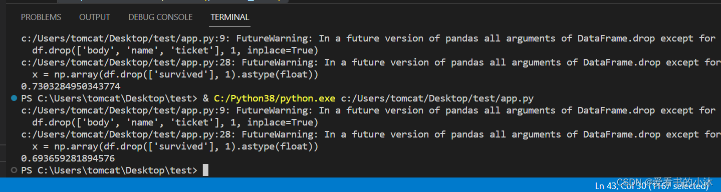
df = pd.read_excel('titanic.xls')
df.drop(['body', 'name', 'ticket'], 1, inplace=True)
df.fillna(0, inplace=True)  # 把NaN替换为0# 把字符串映射为数字，例如{female:1, male:0}
df_map = {}
cols = df.columns.values
for col in cols:if df[col].dtype != np.int64 and df[col].dtype != np.float64:temp = {}x = 0for ele in set(df[col].values.tolist()):if ele not in temp:temp[ele] = xx += 1df_map[df[col].name] = tempdf[col] = list(map(lambda val: temp[val], df[col]))# 将每一列特征标准化为标准正太分布
x = np.array(df.drop(['survived'], 1).astype(float))
x = preprocessing.scale(x)
clf = KMeans(n_clusters=2)
clf.fit(x)# 计算分组准确率
y = np.array(df['survived'])
correct = 0
for i in range(len(x)):predict_data = np.array(x[i].astype(float))predict_data = predict_data.reshape(-1, len(predict_data))predict = clf.predict(predict_data)if predict[0] == y[i]:correct += 1print(correct * 1.0 / len(x))

2.2.3 例子3：手写数字数据分类

"""
===========================================================
A demo of K-Means clustering on the handwritten digits data
===========================================================
"""# %%
# Load the dataset
# ----------------
#
# We will start by loading the `digits` dataset. This dataset contains
# handwritten digits from 0 to 9. In the context of clustering, one would like
# to group images such that the handwritten digits on the image are the same.import numpy as npfrom sklearn.datasets import load_digitsdata, labels = load_digits(return_X_y=True)
(n_samples, n_features), n_digits = data.shape, np.unique(labels).sizeprint(f"# digits: {n_digits}; # samples: {n_samples}; # features {n_features}")# %%
# Define our evaluation benchmark
# -------------------------------
#
# We will first our evaluation benchmark. During this benchmark, we intend to
# compare different initialization methods for KMeans. Our benchmark will:
#
# * create a pipeline which will scale the data using a
#   :class:`~sklearn.preprocessing.StandardScaler`;
# * train and time the pipeline fitting;
# * measure the performance of the clustering obtained via different metrics.
from time import timefrom sklearn import metrics
from sklearn.pipeline import make_pipeline
from sklearn.preprocessing import StandardScalerdef bench_k_means(kmeans, name, data, labels):"""Benchmark to evaluate the KMeans initialization methods.Parameters----------kmeans : KMeans instanceA :class:`~sklearn.cluster.KMeans` instance with the initializationalready set.name : strName given to the strategy. It will be used to show the results in atable.data : ndarray of shape (n_samples, n_features)The data to cluster.labels : ndarray of shape (n_samples,)The labels used to compute the clustering metrics which requires somesupervision."""t0 = time()estimator = make_pipeline(StandardScaler(), kmeans).fit(data)fit_time = time() - t0results = [name, fit_time, estimator[-1].inertia_]# Define the metrics which require only the true labels and estimator# labelsclustering_metrics = [metrics.homogeneity_score,metrics.completeness_score,metrics.v_measure_score,metrics.adjusted_rand_score,metrics.adjusted_mutual_info_score,]results += [m(labels, estimator[-1].labels_) for m in clustering_metrics]# The silhouette score requires the full datasetresults += [metrics.silhouette_score(data,estimator[-1].labels_,metric="euclidean",sample_size=300,)]# Show the resultsformatter_result = ("{:9s}\t{:.3f}s\t{:.0f}\t{:.3f}\t{:.3f}\t{:.3f}\t{:.3f}\t{:.3f}\t{:.3f}")print(formatter_result.format(*results))# %%
# Run the benchmark
# -----------------
#
# We will compare three approaches:
#
# * an initialization using `k-means++`. This method is stochastic and we will
#   run the initialization 4 times;
# * a random initialization. This method is stochastic as well and we will run
#   the initialization 4 times;
# * an initialization based on a :class:`~sklearn.decomposition.PCA`
#   projection. Indeed, we will use the components of the
#   :class:`~sklearn.decomposition.PCA` to initialize KMeans. This method is
#   deterministic and a single initialization suffice.
from sklearn.cluster import KMeans
from sklearn.decomposition import PCAprint(82 * "_")
print("init\t\ttime\tinertia\thomo\tcompl\tv-meas\tARI\tAMI\tsilhouette")kmeans = KMeans(init="k-means++", n_clusters=n_digits, n_init=4, random_state=0)
bench_k_means(kmeans=kmeans, name="k-means++", data=data, labels=labels)kmeans = KMeans(init="random", n_clusters=n_digits, n_init=4, random_state=0)
bench_k_means(kmeans=kmeans, name="random", data=data, labels=labels)pca = PCA(n_components=n_digits).fit(data)
kmeans = KMeans(init=pca.components_, n_clusters=n_digits, n_init=1)
bench_k_means(kmeans=kmeans, name="PCA-based", data=data, labels=labels)print(82 * "_")# %%
# Visualize the results on PCA-reduced data
# -----------------------------------------
#
# :class:`~sklearn.decomposition.PCA` allows to project the data from the
# original 64-dimensional space into a lower dimensional space. Subsequently,
# we can use :class:`~sklearn.decomposition.PCA` to project into a
# 2-dimensional space and plot the data and the clusters in this new space.
import matplotlib.pyplot as pltreduced_data = PCA(n_components=2).fit_transform(data)
kmeans = KMeans(init="k-means++", n_clusters=n_digits, n_init=4)
kmeans.fit(reduced_data)# Step size of the mesh. Decrease to increase the quality of the VQ.
h = 0.02  # point in the mesh [x_min, x_max]x[y_min, y_max].# Plot the decision boundary. For that, we will assign a color to each
x_min, x_max = reduced_data[:, 0].min() - 1, reduced_data[:, 0].max() + 1
y_min, y_max = reduced_data[:, 1].min() - 1, reduced_data[:, 1].max() + 1
xx, yy = np.meshgrid(np.arange(x_min, x_max, h), np.arange(y_min, y_max, h))# Obtain labels for each point in mesh. Use last trained model.
Z = kmeans.predict(np.c_[xx.ravel(), yy.ravel()])# Put the result into a color plot
Z = Z.reshape(xx.shape)
plt.figure(1)
plt.clf()
plt.imshow(Z,interpolation="nearest",extent=(xx.min(), xx.max(), yy.min(), yy.max()),cmap=plt.cm.Paired,aspect="auto",origin="lower",
)plt.plot(reduced_data[:, 0], reduced_data[:, 1], "k.", markersize=2)
# Plot the centroids as a white X
centroids = kmeans.cluster_centers_
plt.scatter(centroids[:, 0],centroids[:, 1],marker="x",s=169,linewidths=3,color="w",zorder=10,
)
plt.title("K-means clustering on the digits dataset (PCA-reduced data)\n""Centroids are marked with white cross"
)
plt.xlim(x_min, x_max)
plt.ylim(y_min, y_max)
plt.xticks(())
plt.yticks(())
plt.show()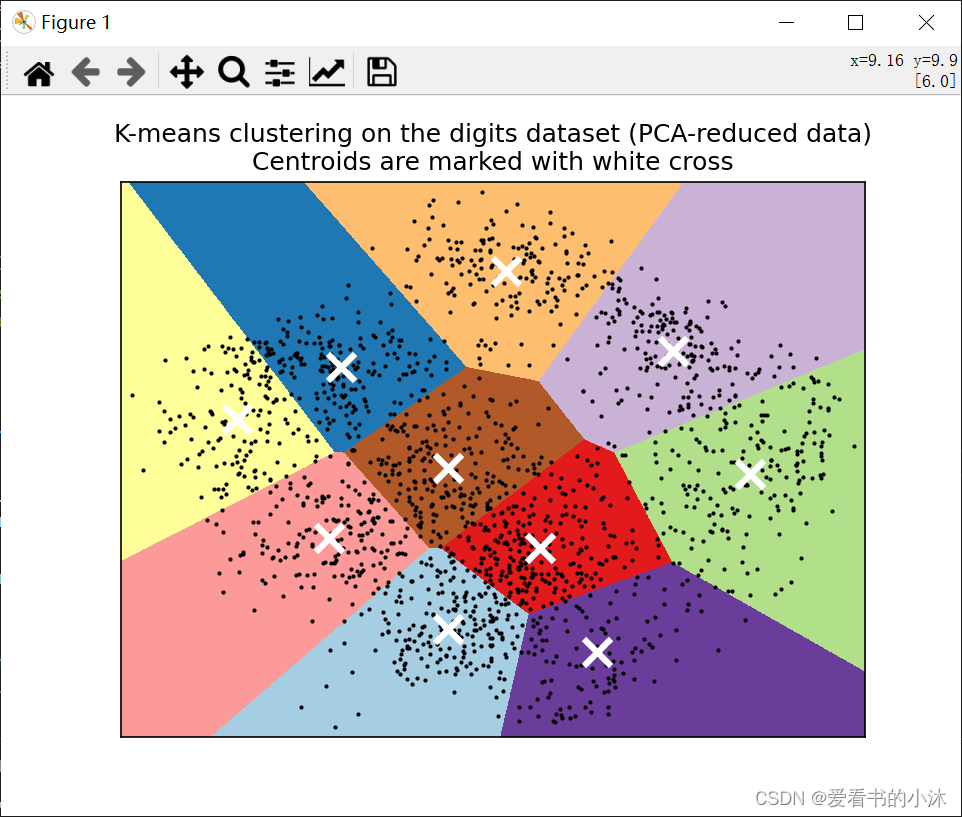

2.2.4 例子4：鸢尾花数据分类

import timeimport pandas as pd
import matplotlib.pyplot as plt
import numpy as np
from numpy import nonzero, array
from sklearn.cluster import KMeans
from sklearn.metrics import f1_score, accuracy_score, normalized_mutual_info_score, rand_score, adjusted_rand_score
from sklearn.preprocessing import LabelEncoder
from sklearn.decomposition import PCA# 数据保存在.csv文件中
iris = pd.read_csv("datasets/data/Iris.csv", header=0)  # 鸢尾花数据集 Iris  class=3
# wine = pd.read_csv("datasets/data/wine.csv")  # 葡萄酒数据集 Wine  class=3
# seeds = pd.read_csv("datasets/data/seeds.csv")  # 小麦种子数据集 seeds  class=3
# wdbc = pd.read_csv("datasets/data/wdbc.csv")  # 威斯康星州乳腺癌数据集 Breast Cancer Wisconsin (Diagnostic)  class=2
# glass = pd.read_csv("datasets/data/glass.csv")  # 玻璃辨识数据集 Glass Identification  class=6
df = iris  # 设置要读取的数据集
# print(df)columns = list(df.columns)  # 获取数据集的第一行，第一行通常为特征名，所以先取出
features = columns[:len(columns) - 1]  # 数据集的特征名（去除了最后一列，因为最后一列存放的是标签，不是数据）
dataset = df[features]  # 预处理之后的数据，去除掉了第一行的数据（因为其为特征名，如果数据第一行不是特征名，可跳过这一步）
attributes = len(df.columns) - 1  # 属性数量（数据集维度）
original_labels = list(df[columns[-1]])  # 原始标签def initialize_centroids(data, k):# 从数据集中随机选择k个点作为初始质心centers = data[np.random.choice(data.shape[0], k, replace=False)]return centersdef get_clusters(data, centroids):# 计算数据点与质心之间的距离，并将数据点分配给最近的质心distances = np.linalg.norm(data[:, np.newaxis] - centroids, axis=2)cluster_labels = np.argmin(distances, axis=1)return cluster_labelsdef update_centroids(data, cluster_labels, k):# 计算每个簇的新质心，即簇内数据点的均值new_centroids = np.array([data[cluster_labels == i].mean(axis=0) for i in range(k)])return new_centroidsdef k_means(data, k, T, epsilon):start = time.time()  # 开始时间，计时# 初始化质心centroids = initialize_centroids(data, k)t = 0while t <= T:# 分配簇cluster_labels = get_clusters(data, centroids)# 更新质心new_centroids = update_centroids(data, cluster_labels, k)# 检查收敛条件if np.linalg.norm(new_centroids - centroids) < epsilon:breakcentroids = new_centroidsprint("第", t, "次迭代")t += 1print("用时：{0}".format(time.time() - start))return cluster_labels, centroids# 计算聚类指标
def clustering_indicators(labels_true, labels_pred):if type(labels_true[0]) != int:labels_true = LabelEncoder().fit_transform(df[columns[len(columns) - 1]])  # 如果数据集的标签为文本类型，把文本标签转换为数字标签f_measure = f1_score(labels_true, labels_pred, average='macro')  # F值accuracy = accuracy_score(labels_true, labels_pred)  # ACCnormalized_mutual_information = normalized_mutual_info_score(labels_true, labels_pred)  # NMIrand_index = rand_score(labels_true, labels_pred)  # RIARI = adjusted_rand_score(labels_true, labels_pred)return f_measure, accuracy, normalized_mutual_information, rand_index, ARI# 绘制聚类结果散点图
def draw_cluster(dataset, centers, labels):center_array = array(centers)if attributes > 2:dataset = PCA(n_components=2).fit_transform(dataset)  # 如果属性数量大于2，降维center_array = PCA(n_components=2).fit_transform(center_array)  # 如果属性数量大于2，降维else:dataset = array(dataset)# 做散点图label = array(labels)plt.scatter(dataset[:, 0], dataset[:, 1], marker='o', c='black', s=7)  # 原图# plt.show()colors = np.array(["#FF0000", "#0000FF", "#00FF00", "#FFFF00", "#00FFFF", "#FF00FF", "#800000", "#008000", "#000080", "#808000","#800080", "#008080", "#444444", "#FFD700", "#008080"])# 循换打印k个簇，每个簇使用不同的颜色for i in range(k):plt.scatter(dataset[nonzero(label == i), 0], dataset[nonzero(label == i), 1], c=colors[i], s=7, marker='o')# plt.scatter(center_array[:, 0], center_array[:, 1], marker='x', color='m', s=30)  # 聚类中心plt.show()if __name__ == "__main__":k = 3  # 聚类簇数T = 100  # 最大迭代数n = len(dataset)  # 样本数epsilon = 1e-5# 预测全部数据# labels, centers = k_means(np.array(dataset), k, T, epsilon)clf = KMeans(n_clusters=k, max_iter=T, tol=epsilon)clf.fit(np.array(dataset))  # 分组centers = clf.cluster_centers_ # 两组数据点的中心点labels = clf.labels_   # 每个数据点所属分组# print(labels)F_measure, ACC, NMI, RI, ARI = clustering_indicators(original_labels, labels)  # 计算聚类指标print("F_measure:", F_measure, "ACC:", ACC, "NMI", NMI, "RI", RI, "ARI", ARI)# print(membership)# print(centers)# print(dataset)draw_cluster(dataset, centers, labels=labels)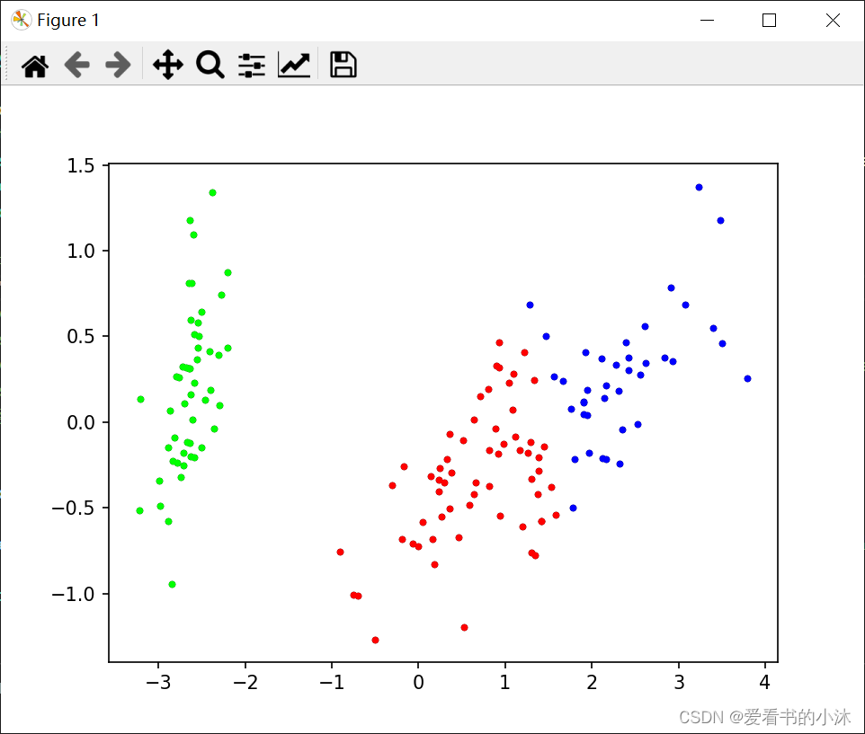

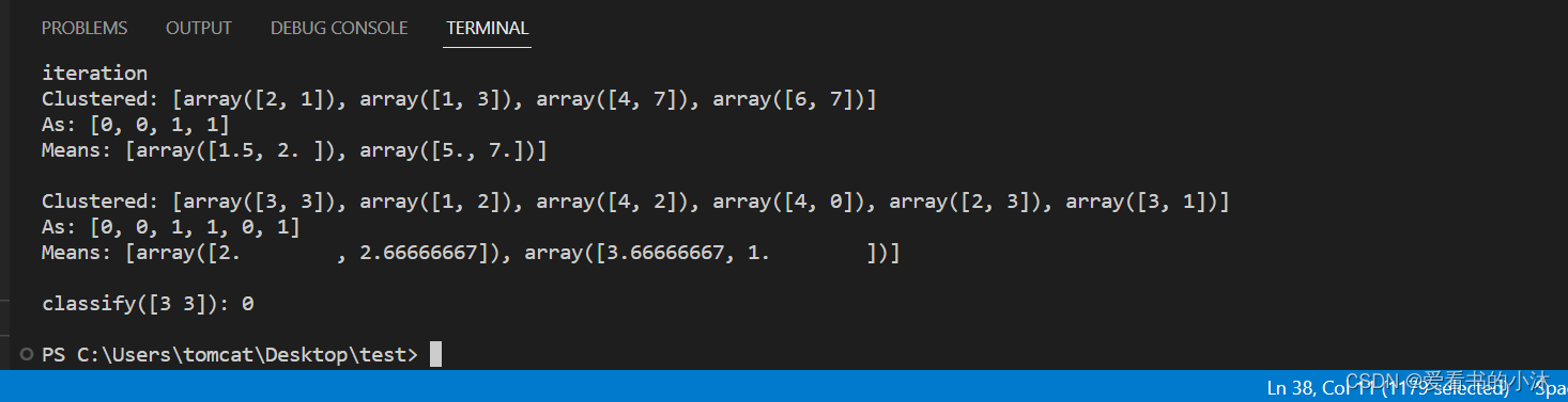
2.3 K-Means（nltk）

https://www.nltk.org/api/nltk.cluster.kmeans.html

K-means 聚类器从 k 个任意选择的均值开始，然后分配 具有最接近均值的聚类的每个向量。然后，它会重新计算 每个簇的均值，作为簇中向量的质心。这 重复该过程，直到群集成员身份稳定下来。这是一个 爬坡算法，可能收敛到局部最大值。因此， 聚类通常以随机的初始均值重复，并且大多数 选择常见的输出均值。

def demo():# example from figure 14.9, page 517, Manning and Schutzeimport numpyfrom nltk.cluster import KMeansClusterer, euclidean_distancevectors = [numpy.array(f) for f in [[2, 1], [1, 3], [4, 7], [6, 7]]]means = [[4, 3], [5, 5]]clusterer = KMeansClusterer(2, euclidean_distance, initial_means=means)clusters = clusterer.cluster(vectors, True, trace=True)print("Clustered:", vectors)print("As:", clusters)print("Means:", clusterer.means())print()vectors = [numpy.array(f) for f in [[3, 3], [1, 2], [4, 2], [4, 0], [2, 3], [3, 1]]]# test k-means using the euclidean distance metric, 2 means and repeat# clustering 10 times with random seedsclusterer = KMeansClusterer(2, euclidean_distance, repeats=10)clusters = clusterer.cluster(vectors, True)print("Clustered:", vectors)print("As:", clusters)print("Means:", clusterer.means())print()# classify a new vectorvector = numpy.array([3, 3])print("classify(%s):" % vector, end=" ")print(clusterer.classify(vector))print()if __name__ == "__main__":demo()

结语

如果您觉得该方法或代码有一点点用处，可以给作者点个赞，或打赏杯咖啡；╮(￣▽￣)╭
如果您感觉方法或代码不咋地//(ㄒoㄒ)//，就在评论处留言，作者继续改进；o_O???
如果您需要相关功能的代码定制化开发，可以留言私信作者；(✿◡‿◡)
感谢各位大佬童鞋们的支持！( ´ ▽´ )ﾉ ( ´ ▽´)っ！！！

这篇关于【小沐学NLP】Python实现K-Means聚类算法（nltk、sklearn）的文章就介绍到这儿，希望我们推荐的文章对编程师们有所帮助！

---