自然激励技术 （NExT） 与特征系统实现算法 （ERA）（Matlab代码实现）

 👨‍🎓个人主页：研学社的博客 

💥💥💞💞欢迎来到本博客❤️❤️💥💥

🏆博主优势：🌞🌞🌞博客内容尽量做到思维缜密，逻辑清晰，为了方便读者。

⛳️座右铭：行百里者，半于九十。

📋📋📋本文目录如下：🎁🎁🎁

目录

💥1 概述

📚2 运行结果

🌈3 Matlab代码实现

🎉4 参考文献

---

💥1 概述

本文使用时域NExT和频域NExT的特征系统实现算法（ERA）的自然激励技术（NExT）。
用于识别受高斯白噪声激励影响的2DOF系统，并增加激励和响应的不确定性（也是高斯白噪声）。

[Result] = NExTTERA（data，refch，maxlags，fs，ncols，nrows，cut，shift，EMAC_option）

输入 ：data：
包含响应数据的数组，其维度为 （nch，Ndata），其中 nch 是通道数。Ndata 是数据
引用的总长度： 参考通道的 vecor .its 维度 （numref，1） 其中 numref 是参考通道
的数量 maxlags： 互相关函数
fs 中的滞后数： 采样频率
ncols： 汉克尔矩阵中的列数（超过 2/3*numref*（maxlags+1） ）nrows： 汉克尔矩阵中的行数（超过 20 * 模式数）

剪切： 截止值=2*模式
数 移位：最后一行和列块中的移位值（增加 EMAC 灵敏度）通常 =10
EMAC_option：如果此值等于 1，则 EMAC 将与列数无关（仅根据可观测性矩阵计算，而不是根据可控性计算）

输出：

结果：结构由以下组件
组成 参数： NaFreq ： 固有频率矢量 阻尼比： 阻尼比矢量

模态形状： 振型矩阵 指标： MAmC ： 模态振幅相干
EMAC： 扩展模态振幅相干
MPC： 模态相位共线性
CMI： 一致模式指示器
部分： 参与因子
矩阵 A、B、C： 离散 A、B 和 C 矩阵

[结果] = NExTFERA（data，refch，window，N，p，fs，ncols，nrows，cut，shift，EMAC_option）

输入：

data：包含响应数据的数组，其维度为 （nch，Ndata），其中 nch 是通道数。Ndata 是数据
的总长度 refch： 参考通道的 vecor .its 尺寸 （numref，1） 其中 numref 是参考通道
的数量 窗口：窗口大小以获得光谱密度
N：窗口数 p：窗口
之间的重叠比率。从 0 到 1
fs： 采样频率
ncols： 汉克尔矩阵中的列数（大于 2/3*数字参考*（ceil（窗口/2+1）-1） ）nrows： 汉克尔矩阵中的行数（超过 20 * 模式数）cut： 截止值=2*模式
数 移位：最后一行和列块中的移位值（增加 EMAC 灵敏度）

通常 =10
EMAC_option：如果此值等于 1，则 EMAC 将与列数无关（仅根据可观测性矩阵计算，而不是根据可控性计算）

输出：

结果：结构由以下组件
组成 参数： NaFreq ： 固有频率矢量 阻尼比： 阻尼比矢量

模态形状： 振型矩阵 指标： MAmC ： 模态振幅相干
EMAC： 扩展模态振幅相干
MPC： 模态相位共线性
CMI： 一致模式指示器
部分： 参与因子
矩阵 A、B、C： 离散 A、B 和 C 矩阵

📚2 运行结果

🌈3 Matlab代码实现

部分代码：

%Apply modal superposition to get response
%--------------------------------------------------------------------------

n=size(f,1);
dt=1/fs; %sampling rate
[Vectors, Values]=eig(K,M);
Freq=sqrt(diag(Values))/(2*pi); % undamped natural frequency
steps=size(f,2);

Mn=diag(Vectors'*M*Vectors); % uncoupled mass
Cn=diag(Vectors'*C*Vectors); % uncoupled damping
Kn=diag(Vectors'*K*Vectors); % uncoupled stifness
wn=sqrt(diag(Values));
zeta=Cn./(sqrt(2.*Mn.*Kn));  % damping ratio
wd=wn.*sqrt(1-zeta.^2);

fn=Vectors'*f; % generalized input force matrix

t=[0:dt:dt*steps-dt];

for i=1:1:n
    
    h(i,:)=(1/(Mn(i)*wd(i))).*exp(-zeta(i)*wn(i)*t).*sin(wd(i)*t); %transfer function of displacement
    hd(i,:)=(1/(Mn(i)*wd(i))).*(-zeta(i).*wn(i).*exp(-zeta(i)*wn(i)*t).*sin(wd(i)*t)+wd(i).*exp(-zeta(i)*wn(i)*t).*cos(wd(i)*t)); %transfer function of velocity
    hdd(i,:)=(1/(Mn(i)*wd(i))).*((zeta(i).*wn(i))^2.*exp(-zeta(i)*wn(i)*t).*sin(wd(i)*t)-zeta(i).*wn(i).*wd(i).*exp(-zeta(i)*wn(i)*t).*cos(wd(i)*t)-wd(i).*((zeta(i).*wn(i)).*exp(-zeta(i)*wn(i)*t).*cos(wd(i)*t))-wd(i)^2.*exp(-zeta(i)*wn(i)*t).*sin(wd(i)*t)); %transfer function of acceleration
    
    qq=conv(fn(i,:),h(i,:))*dt;
    qqd=conv(fn(i,:),hd(i,:))*dt;
    qqdd=conv(fn(i,:),hdd(i,:))*dt;
    
    q(i,:)=qq(1:steps); % modal displacement
    qd(i,:)=qqd(1:steps); % modal velocity
    qdd(i,:)=qqdd(1:steps); % modal acceleration
       
end

x=Vectors*q; %displacement
v=Vectors*qd; %vecloity
a=Vectors*qdd; %vecloity

%Add noise to excitation and response
%--------------------------------------------------------------------------
f2=f+0.1*randn(2,10000);
a2=a+0.1*randn(2,10000);
v2=v+0.1*randn(2,10000);
x2=x+0.1*randn(2,10000);

%Plot displacement of first floor without and with noise
%--------------------------------------------------------------------------
figure;
subplot(3,2,1)
plot(t,f(1,:)); xlabel('Time (sec)');  ylabel('Force1'); title('First Floor');
subplot(3,2,2)
plot(t,f(2,:)); xlabel('Time (sec)');  ylabel('Force2'); title('Second Floor');
subplot(3,2,3)
plot(t,x(1,:)); xlabel('Time (sec)');  ylabel('DSP1');
subplot(3,2,4)
plot(t,x(2,:)); xlabel('Time (sec)');  ylabel('DSP2');
subplot(3,2,5)
plot(t,x2(1,:)); xlabel('Time (sec)');  ylabel('DSP1+Noise');
subplot(3,2,6)
plot(t,x2(2,:)); xlabel('Time (sec)');  ylabel('DSP2+Noise');

%Identify modal parameters using displacement with added uncertainty
%--------------------------------------------------------------------------
data=x2;
refch=2;
maxlags=999;
window=2000;
N=5;
p=0;
ncols=800;    
nrows=200;       
cut=4;        
shift=10;      
EMAC_option=1; 

[Result1] = NExTFERA(data,refch,window,N,p,fs,ncols,nrows,cut,shift,EMAC_option);
[Result2] = NExTTERA(data,refch,maxlags,fs,ncols,nrows,cut,shift,EMAC_option);

%Plot Impulse Response Functions
%--------------------------------------------------------------------------
IRFT= NExTT(data,refch,maxlags);
IRFF= NExTF(data,refch,window,N,p);

t2=[0:dt:999*dt];
figure;
subplot(2,2,1)
plot(t2,IRFT(1,:)); xlabel('Time (sec)');  ylabel('IRF1'); title('NExTT');
subplot(2,2,2)
plot(t2,IRFF(1,:)); xlabel('Time (sec)');  ylabel('IRF1'); title('NExTF');
subplot(2,2,3)
plot(t2,IRFT(2,:)); xlabel('Time (sec)');  ylabel('IRF2');
subplot(2,2,4)
plot(t2,IRFF(2,:)); xlabel('Time (sec)');  ylabel('IRF2');

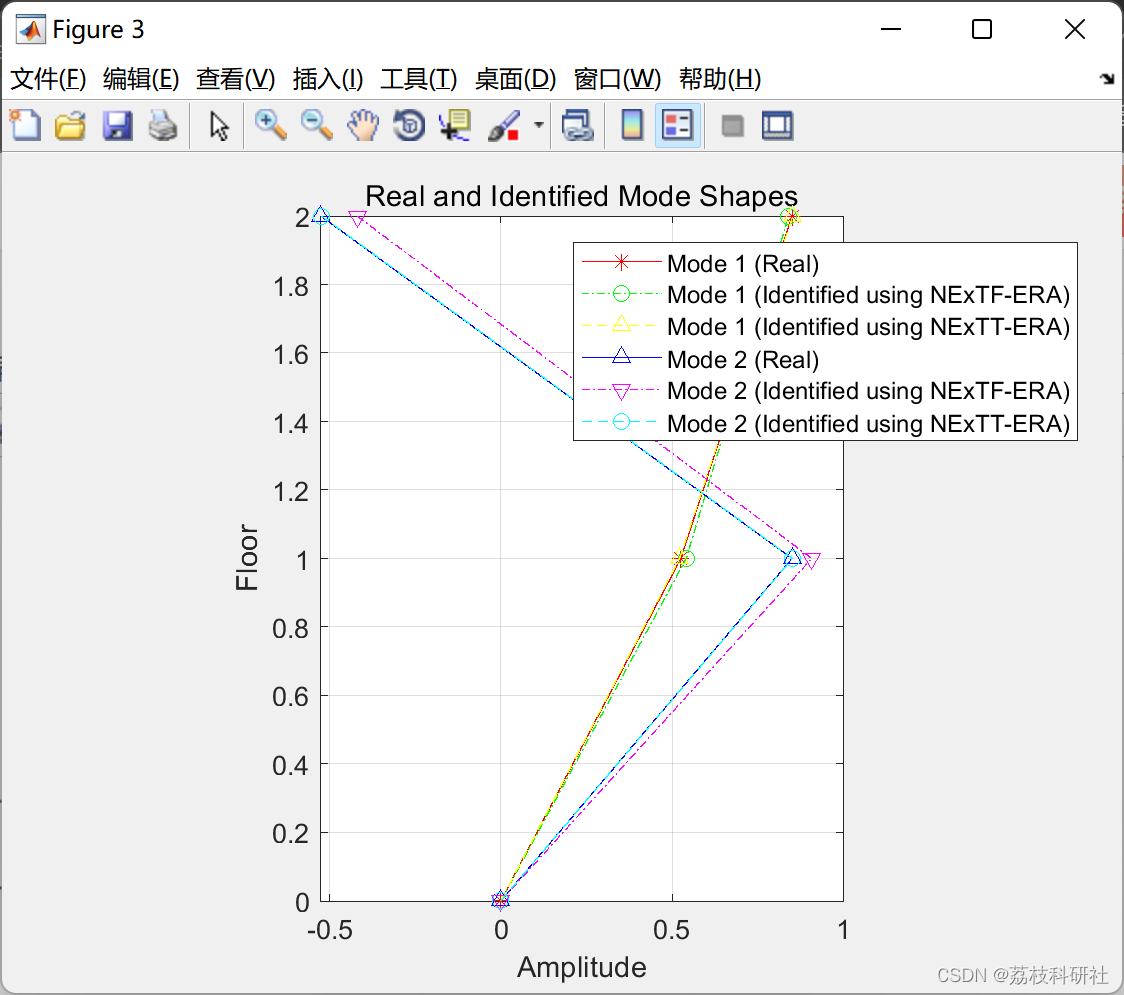
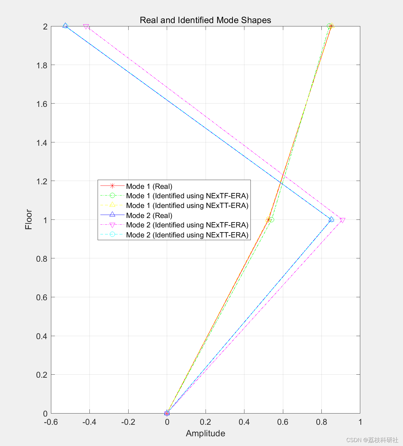
%Plot real and identified first modes to compare between them
%--------------------------------------------------------------------------
figure;
plot([0 ; -Vectors(:,1)],[0 1 2],'r*-');
hold on
plot([0  ;Result1.Parameters.ModeShape(:,1)],[0 1 2],'go-.');
hold on
plot([0  ;Result2.Parameters.ModeShape(:,1)],[0 1 2],'y^--');
hold on
plot([0 ; -Vectors(:,2)],[0 1 2],'b^-');
hold on
plot([0  ;Result1.Parameters.ModeShape(:,2)],[0 1 2],'mv-.');
hold on
plot([0  ;Result2.Parameters.ModeShape(:,2)],[0 1 2],'co--');
hold off
title('Real and Identified Mode Shapes');
legend('Mode 1 (Real)','Mode 1 (Identified using NExTF-ERA)','Mode 1 (Identified using NExTT-ERA)'...
      ,'Mode 2 (Real)','Mode 2 (Identified using NExTF-ERA)','Mode 2 (Identified using NExTT-ERA)');
xlabel('Amplitude');
ylabel('Floor');
grid on;
daspect([1 1 1]);

%Display real and Identified natural frequencies and damping ratios
%--------------------------------------------------------------------------
disp('Real and Identified Natural Drequencies and Damping Ratios of the First Mode'); 
disp(strcat('Real: Frequency=',num2str(Freq(1)),'Hz',' Damping Ratio=',num2str(zeta(1)*100),'%'));
disp(strcat('NExTF-ERA: Frequency=',num2str(Result1.Parameters.NaFreq(1)),'Hz',' Damping Ratio=',num2str(Result1.Parameters.DampRatio(1)),'%'));
disp(strcat('CMI of The Identified Mode=',num2str(Result1.Indicators.CMI(1)),'%'));
disp(strcat('NExTT-ERA: Frequency=',num2str(Result2.Parameters.NaFreq(1)),'Hz',' Damping Ratio=',num2str(Result2.Parameters.DampRatio(1)),'%'));
disp(strcat('CMI of The Identified Mode=',num2str(Result2.Indicators.CMI(1)),'%'));
disp('-----------')

🎉4 参考文献

部分理论来源于网络，如有侵权请联系删除。

[1] R. Pappa, K. Elliott, and A. Schenk, “A consistent-mode indicator for the eigensystem realization algorithm,” Journal of Guidance Control and Dynamics (1993), 1993.

[2] R. S. Pappa, G. H. James, and D. C. Zimmerman, “Autonomous modal identification of the space shuttle tail rudder,” Journal of Spacecraft and Rockets, vol. 35, no. 2, pp. 163–169, 1998.

[3] James, G. H., Thomas G. Carne, and James P. Lauffer. "The natural excitation technique (NExT) for modal parameter extraction from operating structures." Modal Analysis-the International Journal of Analytical and Experimental Modal Analysis 10.4 (1995): 260.

[4] Al Rumaithi, Ayad, "Characterization of Dynamic Structures Using Parametric and Non-parametric System Identification Methods" (2014). Electronic Theses and Dissertations. 1325.

[5] Al-Rumaithi, Ayad, Hae-Bum Yun, and Sami F. Masri. "A Comparative Study of Mode Decomposition to Relate Next-ERA, PCA, and ICA Modes." Model Validation and Uncertainty Quantification, Volume 3. Springer, Cham, 2015. 113-133.