《自然语言处理学习之路》11 文本特征方法对比-词袋，TFIDF，Word2Vec，神经网络模型

书山有路勤为径，学海无涯苦作舟

一、数据预处理与观测

1.1 数据清洗

社交媒体上有些讨论是关于灾难，疾病，暴乱的，有些只是开玩笑或者是电影情节，我们该如何让机器能分辨出这两种讨论呢?

import keras
import nltk
import pandas as pd
import numpy as np
import re
import codecs

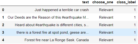
读取数据，并且给行命名

questions = pd.read_csv("socialmedia_relevant_cols_clean.csv")
questions.columns=['text', 'choose_one', 'class_label']
questions.head()

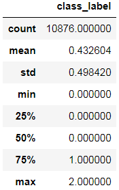
查看导入数据的状态

questions.describe()

数据清洗，去掉无用字符,利用正则,另存为clean_data

def standardize_text(df, text_field):df[text_field] = df[text_field].str.replace(r"http\S+", "")df[text_field] = df[text_field].str.replace(r"http", "")df[text_field] = df[text_field].str.replace(r"@\S+", "")df[text_field] = df[text_field].str.replace(r"[^A-Za-z0-9(),!?@\'\`\"\_\n]", " ")df[text_field] = df[text_field].str.replace(r"@", "at")df[text_field] = df[text_field].str.lower()return dfquestions = standardize_text(questions, "text")questions.to_csv("clean_data.csv")
questions.head()

读取清洗的数据

clean_questions = pd.read_csv("clean_data.csv")
clean_questions.tail()

1.2数据分布情况

看数据时候倾斜，分类任务之前，先观测不同类别的数据是否有倾斜，倾斜的话就选择上采样或者下采样

clean_questions.groupby("class_label").count()

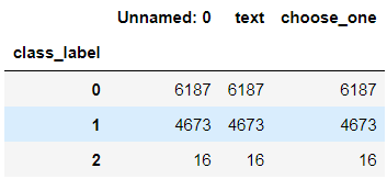
看起来数据还算是均衡的

处理流程

• 分词
• 训练与测试集
• 检查与验证

1.3 分词

这里是用nltk实现英文分词，中文用Jieba分词，将分词结果存到【tokens】这一列

from nltk.tokenize import RegexpTokenizertokenizer = RegexpTokenizer(r'\w+')clean_questions["tokens"] = clean_questions["text"].apply(tokenizer.tokenize)
clean_questions.head()

1.4 统计语料库的单词数，句子长度

统计单词数目

统计句子长度

统计不重复的词数目

from keras.preprocessing.text import Tokenizer
from keras.preprocessing.sequence import pad_sequences
from keras.utils import to_categoricalall_words = [word for tokens in clean_questions["tokens"] for word in tokens]
sentence_lengths = [len(tokens) for tokens in clean_questions["tokens"]]
VOCAB = sorted(list(set(all_words)))
print("%s words total, with a vocabulary size of %s" % (len(all_words), len(VOCAB)))
print("Max sentence length is %s" % max(sentence_lengths))

154724 words total, with a vocabulary size of 18101
Max sentence length is 34

每个文本的长度不一样长，在对于模型的输入，需要是每个样本的长度都是一样长，所以需要设置一个均值的长度，短的就填充，长的就切掉。

句子长度状况

import matplotlib.pyplot as pltfig = plt.figure(figsize=(10, 10)) 
plt.xlabel('Sentence length')
plt.ylabel('Number of sentences')
plt.hist(sentence_lengths)
plt.show()

二、文本特征构建

2.1 词袋模型 Bag of Word Counts

• 先构造语料库去重的所有词的文本矩阵
• 再根据每个文本出现的词频，填充，没有的就是0

from sklearn.model_selection import train_test_split
from sklearn.feature_extraction.text import CountVectorizer, TfidfVectorizerdef cv(data):count_vectorizer = CountVectorizer()emb = count_vectorizer.fit_transform(data)return emb, count_vectorizerlist_corpus = clean_questions["text"].tolist()
list_labels = clean_questions["class_label"].tolist()X_train, X_test, y_train, y_test = train_test_split(list_corpus, list_labels, test_size=0.2, random_state=40)X_train_counts, count_vectorizer = cv(X_train)
X_test_counts = count_vectorizer.transform(X_test)

2.2 PCA展示Bag of Words

将维度的方法有多种PAC，TSNE，LDA，SVD进行降低维度
利用PCA将维度降到2维度

from sklearn.decomposition import PCA, TruncatedSVD
import matplotlib
import matplotlib.patches as mpatchesdef plot_LSA(test_data, test_labels, savepath="PCA_demo.csv", plot=True):lsa = TruncatedSVD(n_components=2)lsa.fit(test_data)lsa_scores = lsa.transform(test_data)color_mapper = {label:idx for idx,label in enumerate(set(test_labels))}color_column = [color_mapper[label] for label in test_labels]colors = ['orange','blue','blue']if plot:plt.scatter(lsa_scores[:,0], lsa_scores[:,1], s=8, alpha=.8, c=color_column, cmap=matplotlib.colors.ListedColormap(colors))red_patch = mpatches.Patch(color='orange', label='Irrelevant')green_patch = mpatches.Patch(color='blue', label='Disaster')plt.legend(handles=[red_patch, green_patch], prop={'size': 30})fig = plt.figure(figsize=(16, 16))          
plot_LSA(X_train_counts, y_train)
plt.show()

基于不同的label画出不同的颜色

但是发现不同维度降低维度，数据都混淆再一起

2.3 逻辑回归建模分类

from sklearn.linear_model import LogisticRegressionclf = LogisticRegression(C=30.0, class_weight='balanced', solver='newton-cg', multi_class='multinomial', n_jobs=-1, random_state=40)
clf.fit(X_train_counts, y_train)y_predicted_counts = clf.predict(X_test_counts)

定义评估方法的函数

from sklearn.metrics import accuracy_score, f1_score, precision_score, recall_score, classification_reportdef get_metrics(y_test, y_predicted):  # true positives / (true positives+false positives)precision = precision_score(y_test, y_predicted, pos_label=None,average='weighted')             # true positives / (true positives + false negatives)recall = recall_score(y_test, y_predicted, pos_label=None,average='weighted')# harmonic mean of precision and recallf1 = f1_score(y_test, y_predicted, pos_label=None, average='weighted')# true positives + true negatives/ totalaccuracy = accuracy_score(y_test, y_predicted)return accuracy, precision, recall, f1accuracy, precision, recall, f1 = get_metrics(y_test, y_predicted_counts)
print("accuracy = %.3f, precision = %.3f, recall = %.3f, f1 = %.3f" % (accuracy, precision, recall, f1))

accuracy = 0.754, precision = 0.752, recall = 0.754, f1 = 0.753

2.4 混淆矩阵检查

import numpy as np
import itertools
from sklearn.metrics import confusion_matrixdef plot_confusion_matrix(cm, classes,normalize=False,title='Confusion matrix',cmap=plt.cm.winter):if normalize:cm = cm.astype('float') / cm.sum(axis=1)[:, np.newaxis]plt.imshow(cm, interpolation='nearest', cmap=cmap)plt.title(title, fontsize=30)plt.colorbar()tick_marks = np.arange(len(classes))plt.xticks(tick_marks, classes, fontsize=20)plt.yticks(tick_marks, classes, fontsize=20)fmt = '.2f' if normalize else 'd'thresh = cm.max() / 2.for i, j in itertools.product(range(cm.shape[0]), range(cm.shape[1])):plt.text(j, i, format(cm[i, j], fmt), horizontalalignment="center", color="white" if cm[i, j] < thresh else "black", fontsize=40)plt.tight_layout()plt.ylabel('True label', fontsize=30)plt.xlabel('Predicted label', fontsize=30)return plt

**传入预测和真实值 **

cm = confusion_matrix(y_test, y_predicted_counts) 
fig = plt.figure(figsize=(10, 10))
plot = plot_confusion_matrix(cm, classes=['Irrelevant','Disaster','Unsure'], normalize=False, title='Confusion matrix')
plt.show()
print(cm)

[[970 251 3]
[274 670 1]
[ 3 4 0]]

发现unsure的数值为0，因为这个分类的数量太少了，机器学习算法会朝着数据方向多的去做

2.5 进一步检查模型的关注点

逻辑回归是：x0w0 + x1w1+···，所以我们可以查看w值的大小，可以看不同分类的哪些词的权重值更大

model.coef 调取w系数 ，构建所有词的与权重的对应关系，再进行排序可视化

def get_most_important_features(vectorizer, model, n=5):index_to_word = {v:k for k,v in vectorizer.vocabulary_.items()}# loop for each classclasses ={}for class_index in range(model.coef_.shape[0]):word_importances = [(el, index_to_word[i]) for i,el in enumerate(model.coef_[class_index])] #去拿系数sorted_coeff = sorted(word_importances, key = lambda x : x[0], reverse=True) #排序tops = sorted(sorted_coeff[:n], key = lambda x : x[0])bottom = sorted_coeff[-n:]classes[class_index] = {'tops':tops,'bottom':bottom}return classesimportance = get_most_important_features(count_vectorizer, clf, 10)

绘图

def plot_important_words(top_scores, top_words, bottom_scores, bottom_words, name):y_pos = np.arange(len(top_words))top_pairs = [(a,b) for a,b in zip(top_words, top_scores)]top_pairs = sorted(top_pairs, key=lambda x: x[1])bottom_pairs = [(a,b) for a,b in zip(bottom_words, bottom_scores)]bottom_pairs = sorted(bottom_pairs, key=lambda x: x[1], reverse=True)top_words = [a[0] for a in top_pairs]top_scores = [a[1] for a in top_pairs]bottom_words = [a[0] for a in bottom_pairs]bottom_scores = [a[1] for a in bottom_pairs]fig = plt.figure(figsize=(10, 10))  plt.subplot(121)plt.barh(y_pos,bottom_scores, align='center', alpha=0.5)plt.title('Irrelevant', fontsize=20)plt.yticks(y_pos, bottom_words, fontsize=14)plt.suptitle('Key words', fontsize=16)plt.xlabel('Importance', fontsize=20)plt.subplot(122)plt.barh(y_pos,top_scores, align='center', alpha=0.5)plt.title('Disaster', fontsize=20)plt.yticks(y_pos, top_words, fontsize=14)plt.suptitle(name, fontsize=16)plt.xlabel('Importance', fontsize=20)plt.subplots_adjust(wspace=0.8)plt.show()top_scores = [a[0] for a in importance[1]['tops']]
top_words = [a[1] for a in importance[1]['tops']]
bottom_scores = [a[0] for a in importance[1]['bottom']]
bottom_words = [a[1] for a in importance[1]['bottom']]plot_important_words(top_scores, top_words, bottom_scores, bottom_words, "Most important words for relevance")

发现模型并没有发现哪些词比较重要，那些词比较不重要，因为词袋模型是基于词频的，就会以频率评判重要性

三、TFIDF Bag of Words

3.1 可视化

TF-IDF不均等对待每个词

def tfidf(data):tfidf_vectorizer = TfidfVectorizer()train = tfidf_vectorizer.fit_transform(data)return train, tfidf_vectorizerX_train_tfidf, tfidf_vectorizer = tfidf(X_train)
X_test_tfidf = tfidf_vectorizer.transform(X_test)

fig = plt.figure(figsize=(16, 16))          
plot_LSA(X_train_tfidf, y_train)
plt.show()

看起来比词频的好那么一点

3.2 逻辑回归建模分类

clf_tfidf = LogisticRegression(C=30.0, class_weight='balanced', solver='newton-cg', multi_class='multinomial', n_jobs=-1, random_state=40)
clf_tfidf.fit(X_train_tfidf, y_train)y_predicted_tfidf = clf_tfidf.predict(X_test_tfidf)

accuracy_tfidf, precision_tfidf, recall_tfidf, f1_tfidf = get_metrics(y_test, y_predicted_tfidf)
print("accuracy = %.3f, precision = %.3f, recall = %.3f, f1 = %.3f" % (accuracy_tfidf, precision_tfidf, recall_tfidf, f1_tfidf))

accuracy = 0.762, precision = 0.760, recall = 0.762, f1 = 0.761

cm2 = confusion_matrix(y_test, y_predicted_tfidf)
fig = plt.figure(figsize=(10, 10))
plot = plot_confusion_matrix(cm2, classes=['Irrelevant','Disaster','Unsure'], normalize=False, title='Confusion matrix')
plt.show()
print("TFIDF confusion matrix")
print(cm2)
print("BoW confusion matrix")
print(cm)

输出：

TFIDF confusion matrix
[[974 249 1]
[261 684 0]
[ 3 4 0]]
BoW confusion matrix
[[970 251 3]
[274 670 1]
[ 3 4 0]]

3.3 词语的解释

importance_tfidf = get_most_important_features(tfidf_vectorizer, clf_tfidf, 10)

top_scores = [a[0] for a in importance_tfidf[1]['tops']]
top_words = [a[1] for a in importance_tfidf[1]['tops']]
bottom_scores = [a[0] for a in importance_tfidf[1]['bottom']]
bottom_words = [a[1] for a in importance_tfidf[1]['bottom']]plot_important_words(top_scores, top_words, bottom_scores, bottom_words, "Most important words for relevance")

这些词看起来比之前强一些了

问题
我们现在考虑的是每一个词基于频率的情况，如果在新的测试环境下有些词变了呢?比如说goog和positive.有些词可能表达的意义差不多但是却长得不一样，这样我们的模型就难捕捉到了。

四、Word2Vec词向量模型

4.1 Word2Vec建模

可以识别同一个语义的不同词可以聚类在一起

拿直接别人训练好的词向量模型进行实验，300维的向量模型

import gensimword2vec_path = "GoogleNews-vectors-negative300.bin"
word2vec = gensim.models.KeyedVectors.load_word2vec_format(word2vec_path, binary=True)

将300维度基于词的向量转换为句子向量，最简单的方法取得平均，300维度的词，每一个维度的值相加取得平均值，表达句子向量。

问题：但是取得平均后，就将每一个词同等对待，并没有体现出一些关键词的重要性。

def get_average_word2vec(tokens_list, vector, generate_missing=False, k=300):if len(tokens_list)<1:return np.zeros(k)if generate_missing:vectorized = [vector[word] if word in vector else np.random.rand(k) for word in tokens_list]else:vectorized = [vector[word] if word in vector else np.zeros(k) for word in tokens_list]length = len(vectorized)summed = np.sum(vectorized, axis=0)averaged = np.divide(summed, length)return averageddef get_word2vec_embeddings(vectors, clean_questions, generate_missing=False):embeddings = clean_questions['tokens'].apply(lambda x: get_average_word2vec(x, vectors, generate_missing=generate_missing))return list(embeddings)

embeddings = get_word2vec_embeddings(word2vec, clean_questions)
X_train_word2vec, X_test_word2vec, y_train_word2vec, y_test_word2vec = train_test_split(embeddings, list_labels, test_size=0.2, random_state=40)

X_train_word2vec[0]

array([ 0.05639939, 0.02053833, 0.07635207, 0.06914993, -0.01007262,
-0.04978943, 0.02546038, -0.06045968, 0.04264323, 0.02419935,
0.00375076, -0.15124639, 0.02915809, -0.01554943, -0.10182699,
0.05523972, 0.00953747, 0.0834525 , 0.00200544, -0.0238909 ,
-0.01706369, 0.09193638, 0.03979783, 0.04899052, 0.04707618,
-0.09235491, -0.10698809, 0.07503255, 0.04905628, -0.01991781,
0.04036749, -0.0117856 , -0.00576346, 0.01624843, -0.01823952,
-0.01545715, 0.06020392, 0.02975609, 0.02211217, 0.07844525,
0.05023847, -0.09430913, 0.20582217, -0.05274091, 0.00881231,
0.04394059, -0.01748512, -0.0403268 , 0.03178769, 0.06038993,
0.03867458, 0.00492932, 0.05121649, 0.01256743, -0.02096994,
0.02814593, -0.06389218, 0.01661319, -0.02686709, -0.07981364,
-0.00288318, 0.07032367, -0.07524182, -0.01155599, -0.0259661 ,
0.00625901, -0.05474758, -0.00059877, -0.01737177, 0.07586161,
0.0273136 , -0.00077093, 0.0752638 , 0.05861119, -0.15668742,
-0.00779506, 0.04997617, 0.08768209, 0.04078311, 0.07749503,
0.02886018, -0.08094715, 0.05818976, -0.02744593, -0.00559489,
-0.00488863, -0.06092762, 0.15089634, -0.02423968, 0.02867635,
0.0041097 , 0.00409226, -0.05106317, -0.0156715 , -0.06731596,
0.00594657, 0.02464658, 0.10740153, 0.0207287 , -0.02535357,
-0.05631002, -0.01714507, -0.04964483, -0.00834728, -0.01148841,
0.04122198, 0.00281052, -0.02053833, 0.01521229, -0.10191563,
-0.07321421, -0.01803589, -0.02788144, 0.00172424, 0.07978603,
-0.01517505, 0.03893743, -0.0548212 , 0.03782436, 0.04642305,
-0.05222284, 0.01304263, -0.06944965, 0.01763625, -0.02670433,
-0.03698331, -0.02478899, -0.06544131, 0.05864679, -0.00175549,
-0.11564055, -0.10066441, -0.04190209, -0.02992467, -0.08564534,
-0.02061244, 0.02688017, -0.0045171 , 0.00165086, 0.10750544,
-0.028361 , -0.03209577, 0.0515936 , -0.04164342, 0.02281843,
0.08524286, -0.10112653, -0.14161319, -0.05427769, -0.01017171,
0.09955125, 0.02694847, -0.0915055 , 0.09549531, -0.0138172 ,
0.01547096, 0.00868443, -0.04557078, -0.00442069, 0.01043919,
-0.00775728, 0.02804129, 0.10577102, 0.07417879, -0.0414545 ,
-0.10446894, 0.07996532, -0.06722441, 0.0636742 , -0.05054583,
-0.11369978, 0.02922131, -0.03643508, -0.09067681, -0.06278338,
-0.01135545, 0.09446498, -0.02156576, 0.00918143, 0.0722787 ,
-0.01088969, 0.03180022, -0.00304031, 0.0532895 , 0.07494827,
-0.02797735, -0.06948853, 0.06283715, 0.10689872, 0.02087112,
0.05185082, 0.06266276, 0.01831927, 0.10564604, 0.00259254,
0.08089193, -0.01426479, 0.00684974, -0.03707304, -0.1198062 ,
-0.05715216, 0.01687549, 0.03455462, -0.08835565, 0.05120559,
-0.06600516, -0.01664807, -0.02856736, 0.02654157, -0.00975818,
-0.03065236, -0.04041981, -0.01071312, -0.05153402, -0.14723714,
-0.00877744, 0.08035714, 0.00351824, -0.10722714, -0.03078206,
-0.00496383, -0.01665388, 0.0004069 , -0.02276175, 0.14360192,
-0.09488932, 0.00554548, 0.13301958, -0.02263096, -0.03730701,
0.03650629, -0.02395339, 0.00687372, -0.02563804, 0.03732518,
-0.02720424, -0.0106114 , -0.05050805, 0.00444685, -0.02968924,
0.07124983, -0.00694057, 0.00107829, -0.08331589, -0.03359186,
0.0081293 , -0.0008138 , 0.01801554, 0.02518827, -0.03804089,
0.06714594, 0.00194731, 0.08901033, 0.06102903, 0.03237479,
-0.05186026, 0.02203078, -0.02689325, -0.01497105, -0.07096935,
0.00406174, 0.03199695, -0.05650693, -0.00124395, 0.08180745,
0.10938081, 0.0316787 , 0.01944987, -0.02388909, 0.00355748,
0.0249256 , 0.00739524, 0.0506243 , -0.01226516, 0.01143035,
-0.09211658, -0.02129836, -0.11622447, -0.04239509, -0.05391511,
-0.00467064, -0.01021031, 0.00030227, 0.12456985, -0.0130964 ,
0.02393832, -0.04647537, 0.06130255, 0.02752686, 0.04820469,
-0.06352307, 0.0357637 , -0.1455921 , 0.01995268, -0.04385739,
-0.03136626, -0.04338237, -0.08235096, 0.02723331, -0.01401483])

word2vec是用神经网络迭代计算出来的，解释性也比较差

4.2 降维可视化

fig = plt.figure(figsize=(16, 16))          
plot_LSA(embeddings, list_labels)
plt.show()

看起来就好多了

4.3 分类评估

clf_w2v = LogisticRegression(C=30.0, class_weight='balanced', solver='newton-cg', multi_class='multinomial', random_state=40)
clf_w2v.fit(X_train_word2vec, y_train_word2vec)
y_predicted_word2vec = clf_w2v.predict(X_test_word2vec)

accuracy_word2vec, precision_word2vec, recall_word2vec, f1_word2vec = get_metrics(y_test_word2vec, y_predicted_word2vec)
print("accuracy = %.3f, precision = %.3f, recall = %.3f, f1 = %.3f" % (accuracy_word2vec, precision_word2vec, recall_word2vec, f1_word2vec))

accuracy = 0.777, precision = 0.776, recall = 0.777, f1 = 0.777

cm_w2v = confusion_matrix(y_test_word2vec, y_predicted_word2vec)
fig = plt.figure(figsize=(10, 10))
plot = plot_confusion_matrix(cm, classes=['Irrelevant','Disaster','Unsure'], normalize=False, title='Confusion matrix')
plt.show()
print("Word2Vec confusion matrix")
print(cm_w2v)
print("TFIDF confusion matrix")
print(cm2)
print("BoW confusion matrix")
print(cm)

F1的值为0.777

Word2Vec confusion matrix
[[980 242 2]
[232 711 2]
[ 2 5 0]]
TFIDF confusion matrix
[[974 249 1]
[261 684 0]
[ 3 4 0]]
BoW confusion matrix
[[970 251 3]
[274 670 1]
[ 3 4 0]]

但是word2Vec就比较难看出来，那些词比较重要。

五、基于深度学习的自然语言处理（CNN和RNN）

5.1 建模

CNN本质上是做出一个图像处理，输入需要是一个图像矩阵，CNN在处理的时候用一个filter，一次滑动指定数量的词，提取这些词的特征。不停的向下面滑动，在不停的滑动过程中，综合的考虑的上下文的信息。
基于图像的方式，提取上下文特征

RNN专门做自然语言处理，输入一般是一个序列。每个词都是一个序列，先考虑第一个词，在处理第二个词的时候，不仅处理第二个词还考虑第一个词的输入。

from keras.preprocessing.text import Tokenizer
from keras.preprocessing.sequence import pad_sequences
from keras.utils import to_categoricalEMBEDDING_DIM = 300
MAX_SEQUENCE_LENGTH = 35
VOCAB_SIZE = len(VOCAB)VALIDATION_SPLIT=.2
tokenizer = Tokenizer(num_words=VOCAB_SIZE)
tokenizer.fit_on_texts(clean_questions["text"].tolist())
sequences = tokenizer.texts_to_sequences(clean_questions["text"].tolist())word_index = tokenizer.word_index
print('Found %s unique tokens.' % len(word_index))cnn_data = pad_sequences(sequences, maxlen=MAX_SEQUENCE_LENGTH)
labels = to_categorical(np.asarray(clean_questions["class_label"]))indices = np.arange(cnn_data.shape[0])
np.random.shuffle(indices)
cnn_data = cnn_data[indices]
labels = labels[indices]
num_validation_samples = int(VALIDATION_SPLIT * cnn_data.shape[0])embedding_weights = np.zeros((len(word_index)+1, EMBEDDING_DIM))
for word,index in word_index.items():embedding_weights[index,:] = word2vec[word] if word in word2vec else np.random.rand(EMBEDDING_DIM)
print(embedding_weights.shape)

Found 19098 unique tokens.
(19099, 300)

5.2 CNN

现在，我们将定义一个简单的卷积神经网络

from keras.layers import Dense, Input, Flatten, Dropout, Merge
from keras.layers import Conv1D, MaxPooling1D, Embedding
from keras.layers import LSTM, Bidirectional
from keras.models import Modeldef ConvNet(embeddings, max_sequence_length, num_words, embedding_dim, labels_index, trainable=False, extra_conv=True):embedding_layer = Embedding(num_words,embedding_dim,weights=[embeddings],input_length=max_sequence_length,trainable=trainable)sequence_input = Input(shape=(max_sequence_length,), dtype='int32')embedded_sequences = embedding_layer(sequence_input)# Yoon Kim model (https://arxiv.org/abs/1408.5882)convs = []filter_sizes = [3,4,5]for filter_size in filter_sizes:l_conv = Conv1D(filters=128, kernel_size=filter_size, activation='relu')(embedded_sequences)l_pool = MaxPooling1D(pool_size=3)(l_conv)convs.append(l_pool)l_merge = Merge(mode='concat', concat_axis=1)(convs)# add a 1D convnet with global maxpooling, instead of Yoon Kim modelconv = Conv1D(filters=128, kernel_size=3, activation='relu')(embedded_sequences)pool = MaxPooling1D(pool_size=3)(conv)if extra_conv==True:x = Dropout(0.5)(l_merge)  else:# Original Yoon Kim modelx = Dropout(0.5)(pool)x = Flatten()(x)x = Dense(128, activation='relu')(x)#x = Dropout(0.5)(x)preds = Dense(labels_index, activation='softmax')(x)model = Model(sequence_input, preds)model.compile(loss='categorical_crossentropy',optimizer='adam',metrics=['acc'])return model

5.3 训练网络

x_train = cnn_data[:-num_validation_samples]
y_train = labels[:-num_validation_samples]
x_val = cnn_data[-num_validation_samples:]
y_val = labels[-num_validation_samples:]model = ConvNet(embedding_weights, MAX_SEQUENCE_LENGTH, len(word_index)+1, EMBEDDING_DIM, len(list(clean_questions["class_label"].unique())), False)

model.fit(x_train, y_train, validation_data=(x_val, y_val), epochs=3, batch_size=128)

Train on 8701 samples, validate on 2175 samples
Epoch 1/3
8701/8701 [] - 11s - loss: 0.5964 - acc: 0.7067 - val_loss: 0.4970 - val_acc: 0.7848
Epoch 2/3
8701/8701 [] - 11s - loss: 0.4434 - acc: 0.8019 - val_loss: 0.4722 - val_acc: 0.8005
Epoch 3/3
8701/8701 [==============================] - 11s - loss: 0.3968 - acc: 0.8283 - val_loss: 0.4985 - val_acc: 0.7880
<keras.callbacks.History at 0x12237bc88>