kaggle之皮肤癌数据的深度学习测试

本文主要是介绍kaggle之皮肤癌数据的深度学习测试，希望对大家解决编程问题提供一定的参考价值，需要的开发者们随着小编来一起学习吧！

kaggle之皮肤癌数据的深度学习测试

近期一直在肝深度学习

很久之前，曾经上手搞过一段时间的深度学习，似乎是做轮胎花纹的识别，当初用的是TensorFlow，CPU版本的，但已经很长时间都没弄过了

现在因为各种原因，不得不重新开始。因为设备限制，深度学习的GPU环境一直没搭好，为了快速开始，不得不继续使用CPU版本

我用的是kaggle提供的皮肤癌的数据集，地址在这里，下载的话，需要注册kaggle，压缩包有5个多G，但是解压后只有2G

我的编译环境是本地Python，版本是3.7，编译器是pycharm

下面就正式开始深度学习测试

一、数据简介

介绍的原文：

About Dataset

Overview

Another more interesting than digit classification dataset to use to get biology and medicine students more excited about machine learning and image processing.

Original Data Source

• Original Challenge: https://challenge2018.isic-archive.com
• https://dataverse.harvard.edu/dataset.xhtml?persistentId=doi:10.7910/DVN/DBW86T
  [1] Noel Codella, Veronica Rotemberg, Philipp Tschandl, M. Emre Celebi, Stephen Dusza, David Gutman, Brian Helba, Aadi Kalloo, Konstantinos Liopyris, Michael Marchetti, Harald Kittler, Allan Halpern: “Skin Lesion Analysis Toward Melanoma Detection 2018: A Challenge Hosted by the International Skin Imaging Collaboration (ISIC)”, 2018; https://arxiv.org/abs/1902.03368

[2] Tschandl, P., Rosendahl, C. & Kittler, H. The HAM10000 dataset, a large collection of multi-source dermatoscopic images of common pigmented skin lesions. Sci. Data 5, 180161 doi:10.1038/sdata.2018.161 (2018).

From Authors

Training of neural networks for automated diagnosis of pigmented skin lesions is hampered by the small size and lack of diversity of available dataset of dermatoscopic images. We tackle this problem by releasing the HAM10000 (“Human Against Machine with 10000 training images”) dataset. We collected dermatoscopic images from different populations, acquired and stored by different modalities. The final dataset consists of 10015 dermatoscopic images which can serve as a training set for academic machine learning purposes. Cases include a representative collection of all important diagnostic categories in the realm of pigmented lesions: Actinic keratoses and intraepithelial carcinoma / Bowen’s disease (akiec), basal cell carcinoma (bcc), benign keratosis-like lesions (solar lentigines / seborrheic keratoses and lichen-planus like keratoses, bkl), dermatofibroma (df), melanoma (mel), melanocytic nevi (nv) and vascular lesions (angiomas, angiokeratomas, pyogenic granulomas and hemorrhage, vasc).

More than 50% of lesions are confirmed through histopathology (histo), the ground truth for the rest of the cases is either follow-up examination (follow_up), expert consensus (consensus), or confirmation by in-vivo confocal microscopy (confocal). The dataset includes lesions with multiple images, which can be tracked by the lesion_id-column within the HAM10000_metadata file.

The test set is not public, but the evaluation server remains running (see the challenge website). Any publications written using the HAM10000 data should be evaluated on the official test set hosted there, so that methods can be fairly compared.

估计大伙儿和我一样，不太乐意看英文，那我大致翻译一下

首先，他说这是另一个比数字分类更有趣的数据集，用来让生物和医学学生对机器学习和图像处理更感兴趣，深度学习一般最先上手的就是手写数字分类了吧

然后，作者介绍说，神经网络用于色素皮肤病变自动诊断的训练由于皮肤镜图像的小尺寸和缺乏多样性数据集而受到阻碍。我们通过发布HAM 10000(“10000训练图像的人对机器”)数据集来解决这个问题。我们收集了不同人群的皮肤镜图像，并以不同的方式获取和存储。最后的数据集由10015张皮肤科图像组成，这些图像可以作为学习机器学习的训练集。病例包括色素沉着病变领域的所有重要诊断类别：光化角化病和上皮内癌/鲍温病(Akiec)、基底细胞癌(BCC)、良性角化样病变(太阳扁桃体/脂溢性角化角化症和扁平苔藓样角化物、BKL)、皮肤纤维瘤(DF)、黑色素瘤(MEL)、黑色素细胞痣(NV)和血管病变(血管瘤、血管瘤、化脓性肉芽肿和出血，VASc)。
超过50%的病变是通过组织病理学(组织病理学)确认的，其余病例的基本真相要么是随访检查(随访)，要么是专家共识(共识)，或者是活体共聚焦显微镜(共聚焦)确认。数据集包含具有多个图像的病变，这些图像可以由HAM 10000_元数据文件中的PAILE_id列跟踪。
测试集是不公开的，但是评估服务器保持运行（参见挑战赛网站）。任何使用HAM10000数据编写的出版物都应该在那里托管的官方测试集上进行评估，以便可以公平地比较各种方法。

全部的数据包括图像数据和文本标签数据，如下：

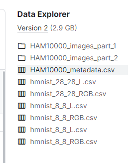
图像数据在俩文件夹中，csv文件是针对不同的数据的特征数据，共有10015张图片

数据简介就这些了，要想看更详细的，可以直接去kaggle上看

二、深度学习建模

建模过程我参考了一个点赞数最多的commit，作者用的是CNN（卷积神经网络），准确率能达到77%

总共有这么几个步骤：

1、导入所需的库

import time
import matplotlib.pyplot as plt
import numpy as np
import pandas as pd
import os
from glob import glob
import seaborn as snssns.set()
from PIL import Imagenp.random.seed(123)
from sklearn.preprocessing import label_binarize
from sklearn.metrics import confusion_matrix
import itertoolsimport keras
from keras.utils.np_utils import to_categorical  # used for converting labels to one-hot-encoding
from keras.models import Sequential
from keras.layers import Dense, Dropout, Flatten, Conv2D, MaxPool2D
from keras import backend as K
import itertools
from keras.layers.normalization import BatchNormalization
from keras.utils.np_utils import to_categorical  # convert to one-hot-encodingfrom keras.optimizers import Adam
from keras.preprocessing.image import ImageDataGenerator
from keras.callbacks import ReduceLROnPlateau
from sklearn.model_selection import train_test_splitstart_time = time.time()

程序跑下来，有些库没有用到，我在作者的基础上，添加了一个计时器，用来计算函数的运行时间

2、制作图像和标签的字典

这一步主要是用来读取数据的

看下面的代码

base_skin_dir = os.path.join('.', 'input')
# base_skin_dir = '.\\input'# Merging images from both folders HAM10000_images_part1.zip and HAM10000_images_part2.zip into one dictionaryimageid_path_dict = {os.path.splitext(os.path.basename(x))[0]: xfor x in glob(os.path.join(base_skin_dir, '*', '*.jpg'))}# This dictionary is useful for displaying more human-friendly labels later onlesion_type_dict = {'nv': 'Melanocytic nevi','mel': 'Melanoma','bkl': 'Benign keratosis-like lesions ','bcc': 'Basal cell carcinoma','akiec': 'Actinic keratoses','vasc': 'Vascular lesions','df': 'Dermatofibroma'
}

注意看一下我的目录结构

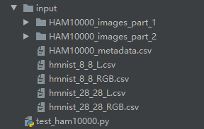
test_ham10000.py就是我的py文件，和input目录同一层级

3、读取特征数据

# 读取数据
skin_df = pd.read_csv(os.path.join(base_skin_dir, 'HAM10000_metadata.csv'))# Creating New Columns for better readabilityskin_df['path'] = skin_df['image_id'].map(imageid_path_dict.get)
skin_df['cell_type'] = skin_df['dx'].map(lesion_type_dict.get)
skin_df['cell_type_idx'] = pd.Categorical(skin_df['cell_type']).codes

这个数据应该是病例数据，包括病例id、图像ID、病例性别、年龄等，然后根据原始数据，创建了其他几个特征

• 根据image_id设置病例的图片路径
• 根据cell_type（细胞类型？）设置dx
• 根据细胞类型设置索引

示例如下：

lesion_id	image_id	dx	dx_type	age	sex	localization	path	cell_type	cell_type_idx
0	HAM_0000118	ISIC_0027419	bkl	histo	80.0	male	scalp	…/input/ham10000_images_part_1/ISIC_0027419.jpg	Benign keratosis-like lesions	2
1	HAM_0000118	ISIC_0025030	bkl	histo	80.0	male	scalp	…/input/ham10000_images_part_1/ISIC_0025030.jpg	Benign keratosis-like lesions	2
2	HAM_0002730	ISIC_0026769	bkl	histo	80.0	male	scalp	…/input/ham10000_images_part_1/ISIC_0026769.jpg	Benign keratosis-like lesions	2
3	HAM_0002730	ISIC_0025661	bkl	histo	80.0	male	scalp	…/input/ham10000_images_part_1/ISIC_0025661.jpg	Benign keratosis-like lesions	2
4	HAM_0001466	ISIC_0031633	bkl	histo	75.0	male	ear	…/input/ham10000_images_part_2/ISIC_0031633.jpg	Benign keratosis-like lesions	2

4、数据清洗

发现skin_df中的年龄存在空值，需要填充一下，用均值填充

skin_df['age'].fillna((skin_df['age'].mean()), inplace=True)

5、数据特征

主要是观察了一下数据的分布特征

# 数据特征
fig, ax1 = plt.subplots(1, 1, figsize=(10, 5))
skin_df['cell_type'].value_counts().plot(kind='bar', ax=ax1)
plt.xticks(rotation=0)
plt.show()
skin_df['dx_type'].value_counts().plot(kind='bar')
plt.show()

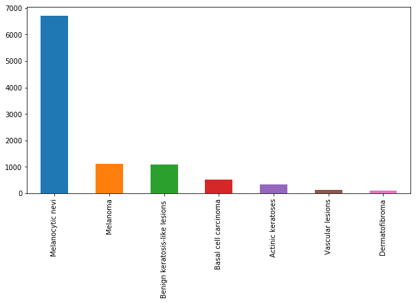
从上面的图中可以看出，与其他类型的细胞相比，黑色素细胞痣的细胞类型有非常多的实例。

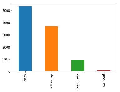
dx_type，以查看其4个类别的分布，如下所示:

1. 组织病理学（Histo）：切除病灶的组织病理学诊断由专门的皮肤病理学家进行。
2. 共焦（confocal）：反射共焦显微术是一种在体成像技术，其分辨率在近细胞水平，有些面部良性，在人工直方图变化前后，所有训练集图像在实验室颜色空间中都有灰色世界的假设。
3. 随访（follow_up）：如果数字皮肤镜监测的痣在3次随访或1.5年的随访中没有显示出任何变化，生物学家接受这一检查作为生物善意的证据。只有痣，但没有其他良性诊断被标记为这种基础真相，因为皮肤科医生通常不监测皮肤病纤维瘤，脂溢性角化，或血管病变。
4. 共识（consensus）：对于典型的无组织病理学或随访的良性病例，生物学家提供作者PT和HK的专家共识评级。只有当两位作者独立地给出相同的明确的良性诊断时，他们才会使用一致的标签。有这种真相的病变通常是出于教育原因而拍摄的，不需要进一步的随访或活检来确认。

非医学专业，看起来实在费劲

还有很多其他的特征，不一一展开了，展开了也看的云里雾里

6、加载并调整图像大小

skin_df['image'] = skin_df['path'].map(lambda x: np.asarray(Image.open(x).resize((100, 75))))# Checking the image size distribution
# skin_df['image'].map(lambda x: x.shape).value_counts()
features = skin_df.drop(columns=['cell_type_idx'], axis=1)
target = skin_df['cell_type_idx']

在此步骤中，图像将从image文件夹中的图像路径加载到名为image的列中。我们还调整图像的大小，图像的原始尺寸为450x600x3，TensorFlow无法处理，所以这就是把它的大小调整为100×75。这里比较耗时，得耐心等待

后面两行就是准备特征数据和目标数据

7、划分训练集和测试集

x_train_o, x_test_o, y_train_o, y_test_o = train_test_split(features, target, test_size=0.20, random_state=1234)

常规操作，机器学习也这么搞

8、数据标准化

x_train = np.asarray(x_train_o['image'].tolist())
x_test = np.asarray(x_test_o['image'].tolist())x_train_mean = np.mean(x_train)
x_train_std = np.std(x_train)x_test_mean = np.mean(x_test)
x_test_std = np.std(x_test)x_train = (x_train - x_train_mean) / x_train_std
x_test = (x_test - x_test_mean) / x_test_std

也是常规操作，计算数据与均值的差，然后除以标准差

9、标签独热编码

这一步我感觉必要性不是特别大

y_train = to_categorical(y_train_o, num_classes=7)
y_test = to_categorical(y_test_o, num_classes=7)

其实就是把数字0-6变成了一个向量，如0->[1,0,0,0,0,0,0]，1->[0,1,0,0,0,0,0]

10、分割训练集和验证集

x_train, x_validate, y_train, y_validate = train_test_split(x_train, y_train, test_size=0.1, random_state=2)

常规操作

11、建模

进入主题，，，

前面就提到了，使用的是CNN

# my CNN architechture is In -> [[Conv2D->relu]*2 -> MaxPool2D -> Dropout]*2 -> Flatten -> Dense -> Dropout -> Out
input_shape = (75, 100, 3)
num_classes = 7model = Sequential()
model.add(Conv2D(32, kernel_size=(3, 3), activation='relu', padding='Same', input_shape=input_shape))
model.add(Conv2D(32, kernel_size=(3, 3), activation='relu', padding='Same', ))
model.add(MaxPool2D(pool_size=(2, 2)))
model.add(Dropout(0.25))model.add(Conv2D(64, (3, 3), activation='relu', padding='Same'))
model.add(Conv2D(64, (3, 3), activation='relu', padding='Same'))
model.add(MaxPool2D(pool_size=(2, 2)))
model.add(Dropout(0.40))model.add(Flatten())
model.add(Dense(128, activation='relu'))
model.add(Dropout(0.5))
model.add(Dense(num_classes, activation='softmax'))
model.summary()

输入size就是图像的size

分类结果是7个

使用的是2D卷积，卷积核大小是3*3

当然，也设置了多种卷积形式

12、设置优化器和退火器

在深度学习中，设置优化器和退火器的作用是优化模型的训练过程。优化器可以帮助调整模型参数以最小化损失函数，而退火器可以逐渐减小学习率以优化模型训练的速度和效果。通过合理选择和调整优化器和退火器，可以提高模型的性能和收敛速度。

optimizer = Adam(lr=0.001, beta_1=0.9, beta_2=0.999, epsilon=None, decay=0.0, amsgrad=False)
# Compile the model
model.compile(optimizer=optimizer, loss="categorical_crossentropy", metrics=["accuracy"])
# Set a learning rate annealer
learning_rate_reduction = ReduceLROnPlateau(monitor='val_acc',patience=3,verbose=1,factor=0.5,min_lr=0.00001)

数据增强。数据增强的目的是通过对原始数据进行一系列变换或操作，生成更多、更多样化的训练样本，以增加模型在数据多样性和复杂性方面的鲁棒性和泛化能力。数据增强可以帮助模型更好地理解数据的特征和模式，并减少过拟合的风险，提高模型在未知数据上的表现。

datagen = ImageDataGenerator(featurewise_center=False,  # set input mean to 0 over the datasetsamplewise_center=False,  # set each sample mean to 0featurewise_std_normalization=False,  # divide inputs by std of the datasetsamplewise_std_normalization=False,  # divide each input by its stdzca_whitening=False,  # apply ZCA whiteningrotation_range=10,  # randomly rotate images in the range (degrees, 0 to 180)zoom_range=0.1,  # Randomly zoom imagewidth_shift_range=0.1,  # randomly shift images horizontally (fraction of total width)height_shift_range=0.1,  # randomly shift images vertically (fraction of total height)horizontal_flip=False,  # randomly flip imagesvertical_flip=False)  # randomly flip images
datagen.fit(x_train)

以上代码使用了ImageDataGenerator来进行数据增强操作，包括旋转、缩放、水平和垂直平移、水平和垂直翻转等多种操作，以生成更多样化的训练样本，提高模型的泛化能力。具体来说，这段代码设置了不进行数据标准化和ZCA白化，但进行了图片旋转、随机缩放、水平和垂直平移以及随机翻转等操作。

13、拟合模型

其实就是用增强后的数据来训练模型

epochs = 50 
batch_size = 10
history = model.fit_generator(datagen.flow(x_train,y_train, batch_size=batch_size),epochs = epochs, validation_data = (x_validate,y_validate),verbose = 1, steps_per_epoch=x_train.shape[0] // batch_size, callbacks=[learning_rate_reduction])

在每个epoch内，从生成的增强数据流(datagen.flow)中获取批量大小为10的数据进行训练，训练50个epoch。

同时，在训练过程中使用验证集(x_validate, y_validate)对模型进行验证，以便监控模型性能。steps_per_epoch参数指定每个epoch包含的训练步数，这里是整个训练集的样本数除以批量大小。callbacks参数中传入了learning_rate_reduction回调函数，用于动态调整学习率，以提高模型的性能和收敛速度。

模型跑的很忙，而且直接跑满了我的CPU，看来没有GPU确实不太行，程序运行过程中，我看了一下我的CPU运行情况，几乎一直处于拉满状态

14、模型评估

经过漫长的计算，耗时大概俩小时，终于计算出结果了，赶紧计算一下模型的准确率

loss, accuracy = model.evaluate(x_test, y_test, verbose=1)
loss_v, accuracy_v = model.evaluate(x_validate, y_validate, verbose=1)
print("Validation: accuracy = %f  ;  loss_v = %f" % (accuracy_v, loss_v))
print("Test: accuracy = %f  ;  loss = %f" % (accuracy, loss))
model.save("model.h5")

计算结果：

2003/2003 [==============================] - 1s 694us/step
802/802 [==============================] - 0s 527us/step
Validation: accuracy = 0.785536  ;  loss_v = 0.586728
Test: accuracy = 0.764853  ;  loss = 0.616134

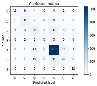
当然也可以看一下模型的学习曲线和损失函数以及混淆矩阵，这里我直接用作者提供的了

三、结语

模型对基底细胞癌的错误预测最多，编码为3，其次是血管病变编码为5。黑素细胞痣编码为0，光化性角化病编码为4，误分率最低。
还可以进一步调整我们的模型，使之更容易达到80%以上的精度。不过77.0344%的预测结果与人眼相比，该模型仍然是有效的。

四、完整代码

#!/usr/bin/env python
# -*- coding:utf-8 -*-
# author:HP
# datetime:2024/4/26 9:40
import time
import matplotlib.pyplot as plt
import numpy as np
import pandas as pd
import os
from glob import glob
import seaborn as snssns.set()
from PIL import Imagenp.random.seed(123)
from sklearn.preprocessing import label_binarize
from sklearn.metrics import confusion_matrix
import itertoolsimport keras
from keras.utils.np_utils import to_categorical  # used for converting labels to one-hot-encoding
from keras.models import Sequential
from keras.layers import Dense, Dropout, Flatten, Conv2D, MaxPool2D
from keras import backend as K
import itertools
from keras.layers.normalization import BatchNormalization
from keras.utils.np_utils import to_categorical  # convert to one-hot-encodingfrom keras.optimizers import Adam
from keras.preprocessing.image import ImageDataGenerator
from keras.callbacks import ReduceLROnPlateau
from sklearn.model_selection import train_test_splitstart_time = time.time()def plot_model_history(model_history):fig, axs = plt.subplots(1, 2, figsize=(15, 5))# summarize history for accuracyaxs[0].plot(range(1, len(model_history.history['acc']) + 1), model_history.history['acc'])axs[0].plot(range(1, len(model_history.history['val_acc']) + 1), model_history.history['val_acc'])axs[0].set_title('Model Accuracy')axs[0].set_ylabel('Accuracy')axs[0].set_xlabel('Epoch')axs[0].set_xticks(np.arange(1, len(model_history.history['acc']) + 1), len(model_history.history['acc']) / 10)axs[0].legend(['train', 'val'], loc='best')# summarize history for lossaxs[1].plot(range(1, len(model_history.history['loss']) + 1), model_history.history['loss'])axs[1].plot(range(1, len(model_history.history['val_loss']) + 1), model_history.history['val_loss'])axs[1].set_title('Model Loss')axs[1].set_ylabel('Loss')axs[1].set_xlabel('Epoch')axs[1].set_xticks(np.arange(1, len(model_history.history['loss']) + 1), len(model_history.history['loss']) / 10)axs[1].legend(['train', 'val'], loc='best')plt.show()base_skin_dir = os.path.join('.', 'input')
# base_skin_dir = '.\\input'# Merging images from both folders HAM10000_images_part1.zip and HAM10000_images_part2.zip into one dictionaryimageid_path_dict = {os.path.splitext(os.path.basename(x))[0]: xfor x in glob(os.path.join(base_skin_dir, '*', '*.jpg'))}# This dictionary is useful for displaying more human-friendly labels later onlesion_type_dict = {'nv': 'Melanocytic nevi','mel': 'Melanoma','bkl': 'Benign keratosis-like lesions ','bcc': 'Basal cell carcinoma','akiec': 'Actinic keratoses','vasc': 'Vascular lesions','df': 'Dermatofibroma'
}# 读取数据
skin_df = pd.read_csv(os.path.join(base_skin_dir, 'HAM10000_metadata.csv'))# Creating New Columns for better readabilityskin_df['path'] = skin_df['image_id'].map(imageid_path_dict.get)
skin_df['cell_type'] = skin_df['dx'].map(lesion_type_dict.get)
skin_df['cell_type_idx'] = pd.Categorical(skin_df['cell_type']).codes# 数据清洗
skin_df['age'].fillna((skin_df['age'].mean()), inplace=True)# 数据特征
fig, ax1 = plt.subplots(1, 1, figsize=(10, 5))
skin_df['cell_type'].value_counts().plot(kind='bar', ax=ax1)
plt.xticks(rotation=0)
plt.show()
skin_df['dx_type'].value_counts().plot(kind='bar')
plt.show()# 加载并调整图像大小
skin_df['image'] = skin_df['path'].map(lambda x: np.asarray(Image.open(x).resize((100, 75))))# Checking the image size distribution
# skin_df['image'].map(lambda x: x.shape).value_counts()
features = skin_df.drop(columns=['cell_type_idx'], axis=1)
target = skin_df['cell_type_idx']# 划分训练集和测试集
x_train_o, x_test_o, y_train_o, y_test_o = train_test_split(features, target, test_size=0.20, random_state=1234)# 数据标准化
x_train = np.asarray(x_train_o['image'].tolist())
x_test = np.asarray(x_test_o['image'].tolist())x_train_mean = np.mean(x_train)
x_train_std = np.std(x_train)x_test_mean = np.mean(x_test)
x_test_std = np.std(x_test)x_train = (x_train - x_train_mean) / x_train_std
x_test = (x_test - x_test_mean) / x_test_std# 标签编码
# Perform one-hot encoding on the labels
y_train = to_categorical(y_train_o, num_classes=7)
y_test = to_categorical(y_test_o, num_classes=7)# 分割训练和验证
x_train, x_validate, y_train, y_validate = train_test_split(x_train, y_train, test_size=0.1, random_state=2)# ！！建模
# Set the CNN model
# my CNN architechture is In -> [[Conv2D->relu]*2 -> MaxPool2D -> Dropout]*2 -> Flatten -> Dense -> Dropout -> Out
input_shape = (75, 100, 3)
num_classes = 7model = Sequential()
model.add(Conv2D(32, kernel_size=(3, 3), activation='relu', padding='Same', input_shape=input_shape))
model.add(Conv2D(32, kernel_size=(3, 3), activation='relu', padding='Same', ))
model.add(MaxPool2D(pool_size=(2, 2)))
model.add(Dropout(0.25))model.add(Conv2D(64, (3, 3), activation='relu', padding='Same'))
model.add(Conv2D(64, (3, 3), activation='relu', padding='Same'))
model.add(MaxPool2D(pool_size=(2, 2)))
model.add(Dropout(0.40))model.add(Flatten())
model.add(Dense(128, activation='relu'))
model.add(Dropout(0.5))
model.add(Dense(num_classes, activation='softmax'))
model.summary()# 设置优化器和退火器
# Define the optimizer
optimizer = Adam(lr=0.001, beta_1=0.9, beta_2=0.999, epsilon=None, decay=0.0, amsgrad=False)
# Compile the model
model.compile(optimizer=optimizer, loss="categorical_crossentropy", metrics=["accuracy"])
# Set a learning rate annealer
learning_rate_reduction = ReduceLROnPlateau(monitor='val_acc',patience=3,verbose=1,factor=0.5,min_lr=0.00001)# 数据增强
datagen = ImageDataGenerator(featurewise_center=False,  # set input mean to 0 over the datasetsamplewise_center=False,  # set each sample mean to 0featurewise_std_normalization=False,  # divide inputs by std of the datasetsamplewise_std_normalization=False,  # divide each input by its stdzca_whitening=False,  # apply ZCA whiteningrotation_range=10,  # randomly rotate images in the range (degrees, 0 to 180)zoom_range=0.1,  # Randomly zoom imagewidth_shift_range=0.1,  # randomly shift images horizontally (fraction of total width)height_shift_range=0.1,  # randomly shift images vertically (fraction of total height)horizontal_flip=False,  # randomly flip imagesvertical_flip=False)  # randomly flip imagesdatagen.fit(x_train)# 模型拟合训练
# Fit the model
epochs = 50
batch_size = 10
history = model.fit_generator(datagen.flow(x_train, y_train, batch_size=batch_size),epochs=epochs, validation_data=(x_validate, y_validate),verbose=1, steps_per_epoch=x_train.shape[0] // batch_size, callbacks=[learning_rate_reduction])# 模型评估
loss, accuracy = model.evaluate(x_test, y_test, verbose=1)
loss_v, accuracy_v = model.evaluate(x_validate, y_validate, verbose=1)
print("Validation: accuracy = %f  ;  loss_v = %f" % (accuracy_v, loss_v))
print("Test: accuracy = %f  ;  loss = %f" % (accuracy, loss))
model.save("model.h5")
plot_model_history(history)end_time = time.time()
run_time = end_time - start_time
print(f"程序运行时间为: {run_time} 秒")

这篇关于kaggle之皮肤癌数据的深度学习测试的文章就介绍到这儿，希望我们推荐的文章对编程师们有所帮助！

---