本文主要是介绍政安晨:【Keras机器学习示例演绎】(九)—— 利用 PointNet 进行点云分类,希望对大家解决编程问题提供一定的参考价值,需要的开发者们随着小编来一起学习吧!
目录
点云分类
建立模型
训练模型
可视化预测
政安晨的个人主页:政安晨
欢迎 👍点赞✍评论⭐收藏
收录专栏: TensorFlow与Keras机器学习实战
希望政安晨的博客能够对您有所裨益,如有不足之处,欢迎在评论区提出指正!
本文目标:用于 ModelNet10 分类的 PointNet 实现。
点云分类
简介
无序三维点集(即点云)的分类、检测和分割是计算机视觉领域的核心问题。本示例实现了开创性的点云深度学习论文 PointNet(Qi 等人,2017 年)。
设置
如果使用 colab,首先使用 !pip install trimesh 安装 trimesh。
import os
import glob
import trimesh
import numpy as np
from tensorflow import data as tf_data
from keras import ops
import keras
from keras import layers
from matplotlib import pyplot as pltkeras.utils.set_random_seed(seed=42)
加载数据集
我们使用 ModelNet10 模型数据集,它是 ModelNet40 数据集的较小 10 类版本。
首先下载数据:
DATA_DIR = keras.utils.get_file("modelnet.zip","http://3dvision.princeton.edu/projects/2014/3DShapeNets/ModelNet10.zip",extract=True,
)
DATA_DIR = os.path.join(os.path.dirname(DATA_DIR), "ModelNet10")
Downloading data from http://3dvision.princeton.edu/projects/2014/3DShapeNets/ModelNet10.zip我们可以使用 trimesh 软件包来读取 .off 网格文件并将其可视化。
mesh = trimesh.load(os.path.join(DATA_DIR, "chair/train/chair_0001.off"))
mesh.show()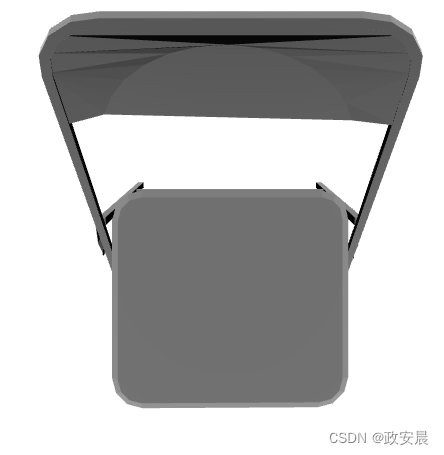
使用这个方法,可以用三维的方式查看。
要将网格文件转换为点云,我们首先需要对网格表面的点进行采样。.sample() 可以执行均匀随机抽样。这里我们对 2048 个位置进行采样,并在 matplotlib 中进行可视化。
points = mesh.sample(2048)fig = plt.figure(figsize=(5, 5))
ax = fig.add_subplot(111, projection="3d")
ax.scatter(points[:, 0], points[:, 1], points[:, 2])
ax.set_axis_off()
plt.show()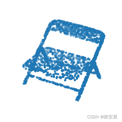
要生成 tf.data.Dataset(),我们首先需要解析 ModelNet 数据文件夹。在将每个网格添加到标准 python 列表并转换为 numpy 数组之前,我们会将其加载并采样为点云。我们还将当前的枚举索引值存储为对象标签,并在以后使用字典调用。
def parse_dataset(num_points=2048):train_points = []train_labels = []test_points = []test_labels = []class_map = {}folders = glob.glob(os.path.join(DATA_DIR, "[!README]*"))for i, folder in enumerate(folders):print("processing class: {}".format(os.path.basename(folder)))# store folder name with ID so we can retrieve laterclass_map[i] = folder.split("/")[-1]# gather all filestrain_files = glob.glob(os.path.join(folder, "train/*"))test_files = glob.glob(os.path.join(folder, "test/*"))for f in train_files:train_points.append(trimesh.load(f).sample(num_points))train_labels.append(i)for f in test_files:test_points.append(trimesh.load(f).sample(num_points))test_labels.append(i)return (np.array(train_points),np.array(test_points),np.array(train_labels),np.array(test_labels),class_map,)设置采样点数和批量大小,并解析数据集。这可能需要 ~5 分钟才能完成。
num_points = 204
NUM_POINTS = 2048
NUM_CLASSES = 10
BATCH_SIZE = 32train_points, test_points, train_labels, test_labels, CLASS_MAP = parse_dataset(NUM_POINTS
)
演绎展示:
processing class: bathtubprocessing class: monitorprocessing class: deskprocessing class: dresserprocessing class: toiletprocessing class: bedprocessing class: sofaprocessing class: chairprocessing class: night_standprocessing class: table现在我们可以将数据读入 tf.data.Dataset() 对象。我们将洗牌缓冲区的大小设置为数据集的整个大小,因为在此之前,数据是按类排序的。在处理点云数据时,数据增强非常重要。我们创建了一个增强函数来抖动和洗牌训练数据集。
def augment(points, label):# jitter pointspoints += keras.random.uniform(points.shape, -0.005, 0.005, dtype="float64")# shuffle pointspoints = keras.random.shuffle(points)return points, labeltrain_size = 0.8
dataset = tf_data.Dataset.from_tensor_slices((train_points, train_labels))
test_dataset = tf_data.Dataset.from_tensor_slices((test_points, test_labels))
train_dataset_size = int(len(dataset) * train_size)dataset = dataset.shuffle(len(train_points)).map(augment)
test_dataset = test_dataset.shuffle(len(test_points)).batch(BATCH_SIZE)train_dataset = dataset.take(train_dataset_size).batch(BATCH_SIZE)
validation_dataset = dataset.skip(train_dataset_size).batch(BATCH_SIZE)
建立模型
每个卷积层和全连接层(末端层除外)都由卷积/密集 -> 批量归一化 -> ReLU 激活组成。
def conv_bn(x, filters):x = layers.Conv1D(filters, kernel_size=1, padding="valid")(x)x = layers.BatchNormalization(momentum=0.0)(x)return layers.Activation("relu")(x)def dense_bn(x, filters):x = layers.Dense(filters)(x)x = layers.BatchNormalization(momentum=0.0)(x)return layers.Activation("relu")(x)PointNet 由两个核心部分组成。主要的 MLP 网络和变压器网络(T-net)。T-net 的目的是通过自己的迷你网络学习仿射变换矩阵。T 网络会使用两次。第一次是将输入特征(n,3)转换为规范表示。第二次是在特征空间(n,3)中进行仿射变换对齐。根据最初的论文,我们限制变换接近正交矩阵(即 ||X*X^T - I|| = 0)。
class OrthogonalRegularizer(keras.regularizers.Regularizer):def __init__(self, num_features, l2reg=0.001):self.num_features = num_featuresself.l2reg = l2regself.eye = ops.eye(num_features)def __call__(self, x):x = ops.reshape(x, (-1, self.num_features, self.num_features))xxt = ops.tensordot(x, x, axes=(2, 2))xxt = ops.reshape(xxt, (-1, self.num_features, self.num_features))return ops.sum(self.l2reg * ops.square(xxt - self.eye))这样,我们就可以定义一个通用函数来构建 T 网层。
def tnet(inputs, num_features):# Initialise bias as the identity matrixbias = keras.initializers.Constant(np.eye(num_features).flatten())reg = OrthogonalRegularizer(num_features)x = conv_bn(inputs, 32)x = conv_bn(x, 64)x = conv_bn(x, 512)x = layers.GlobalMaxPooling1D()(x)x = dense_bn(x, 256)x = dense_bn(x, 128)x = layers.Dense(num_features * num_features,kernel_initializer="zeros",bias_initializer=bias,activity_regularizer=reg,)(x)feat_T = layers.Reshape((num_features, num_features))(x)# Apply affine transformation to input featuresreturn layers.Dot(axes=(2, 1))([inputs, feat_T])主网络可以用同样的方式实现,其中的 t-net 迷你模型可以放在图中的某一层。在这里,我们复制了原始论文中发表的网络架构,但由于使用的是较小的 10 类 ModelNet 数据集,因此每层的权重数量减半。
inputs = keras.Input(shape=(NUM_POINTS, 3))x = tnet(inputs, 3)
x = conv_bn(x, 32)
x = conv_bn(x, 32)
x = tnet(x, 32)
x = conv_bn(x, 32)
x = conv_bn(x, 64)
x = conv_bn(x, 512)
x = layers.GlobalMaxPooling1D()(x)
x = dense_bn(x, 256)
x = layers.Dropout(0.3)(x)
x = dense_bn(x, 128)
x = layers.Dropout(0.3)(x)outputs = layers.Dense(NUM_CLASSES, activation="softmax")(x)model = keras.Model(inputs=inputs, outputs=outputs, name="pointnet")
model.summary()
Model: "pointnet"┏━━━━━━━━━━━━━━━━━━━━━┳━━━━━━━━━━━━━━━━━━━┳━━━━━━━━━┳━━━━━━━━━━━━━━━━━━━━━━┓ ┃ Layer (type) ┃ Output Shape ┃ Param # ┃ Connected to ┃ ┡━━━━━━━━━━━━━━━━━━━━━╇━━━━━━━━━━━━━━━━━━━╇━━━━━━━━━╇━━━━━━━━━━━━━━━━━━━━━━┩ │ input_layer │ (None, 2048, 3) │ 0 │ - │ │ (InputLayer) │ │ │ │ ├─────────────────────┼───────────────────┼─────────┼──────────────────────┤ │ conv1d (Conv1D) │ (None, 2048, 32) │ 128 │ input_layer[0][0] │ ├─────────────────────┼───────────────────┼─────────┼──────────────────────┤ │ batch_normalization │ (None, 2048, 32) │ 128 │ conv1d[0][0] │ │ (BatchNormalizatio… │ │ │ │ ├─────────────────────┼───────────────────┼─────────┼──────────────────────┤ │ activation │ (None, 2048, 32) │ 0 │ batch_normalization… │ │ (Activation) │ │ │ │ ├─────────────────────┼───────────────────┼─────────┼──────────────────────┤ │ conv1d_1 (Conv1D) │ (None, 2048, 64) │ 2,112 │ activation[0][0] │ ├─────────────────────┼───────────────────┼─────────┼──────────────────────┤ │ batch_normalizatio… │ (None, 2048, 64) │ 256 │ conv1d_1[0][0] │ │ (BatchNormalizatio… │ │ │ │ ├─────────────────────┼───────────────────┼─────────┼──────────────────────┤ │ activation_1 │ (None, 2048, 64) │ 0 │ batch_normalization… │ │ (Activation) │ │ │ │ ├─────────────────────┼───────────────────┼─────────┼──────────────────────┤ │ conv1d_2 (Conv1D) │ (None, 2048, 512) │ 33,280 │ activation_1[0][0] │ ├─────────────────────┼───────────────────┼─────────┼──────────────────────┤ │ batch_normalizatio… │ (None, 2048, 512) │ 2,048 │ conv1d_2[0][0] │ │ (BatchNormalizatio… │ │ │ │ ├─────────────────────┼───────────────────┼─────────┼──────────────────────┤ │ activation_2 │ (None, 2048, 512) │ 0 │ batch_normalization… │ │ (Activation) │ │ │ │ ├─────────────────────┼───────────────────┼─────────┼──────────────────────┤ │ global_max_pooling… │ (None, 512) │ 0 │ activation_2[0][0] │ │ (GlobalMaxPooling1… │ │ │ │ ├─────────────────────┼───────────────────┼─────────┼──────────────────────┤ │ dense (Dense) │ (None, 256) │ 131,328 │ global_max_pooling1… │ ├─────────────────────┼───────────────────┼─────────┼──────────────────────┤ │ batch_normalizatio… │ (None, 256) │ 1,024 │ dense[0][0] │ │ (BatchNormalizatio… │ │ │ │ ├─────────────────────┼───────────────────┼─────────┼──────────────────────┤ │ activation_3 │ (None, 256) │ 0 │ batch_normalization… │ │ (Activation) │ │ │ │ ├─────────────────────┼───────────────────┼─────────┼──────────────────────┤ │ dense_1 (Dense) │ (None, 128) │ 32,896 │ activation_3[0][0] │ ├─────────────────────┼───────────────────┼─────────┼──────────────────────┤ │ batch_normalizatio… │ (None, 128) │ 512 │ dense_1[0][0] │ │ (BatchNormalizatio… │ │ │ │ ├─────────────────────┼───────────────────┼─────────┼──────────────────────┤ │ activation_4 │ (None, 128) │ 0 │ batch_normalization… │ │ (Activation) │ │ │ │ ├─────────────────────┼───────────────────┼─────────┼──────────────────────┤ │ dense_2 (Dense) │ (None, 9) │ 1,161 │ activation_4[0][0] │ ├─────────────────────┼───────────────────┼─────────┼──────────────────────┤ │ reshape (Reshape) │ (None, 3, 3) │ 0 │ dense_2[0][0] │ ├─────────────────────┼───────────────────┼─────────┼──────────────────────┤ │ dot (Dot) │ (None, 2048, 3) │ 0 │ input_layer[0][0], │ │ │ │ │ reshape[0][0] │ ├─────────────────────┼───────────────────┼─────────┼──────────────────────┤ │ conv1d_3 (Conv1D) │ (None, 2048, 32) │ 128 │ dot[0][0] │ ├─────────────────────┼───────────────────┼─────────┼──────────────────────┤ │ batch_normalizatio… │ (None, 2048, 32) │ 128 │ conv1d_3[0][0] │ │ (BatchNormalizatio… │ │ │ │ ├─────────────────────┼───────────────────┼─────────┼──────────────────────┤ │ activation_5 │ (None, 2048, 32) │ 0 │ batch_normalization… │ │ (Activation) │ │ │ │ ├─────────────────────┼───────────────────┼─────────┼──────────────────────┤ │ conv1d_4 (Conv1D) │ (None, 2048, 32) │ 1,056 │ activation_5[0][0] │ ├─────────────────────┼───────────────────┼─────────┼──────────────────────┤ │ batch_normalizatio… │ (None, 2048, 32) │ 128 │ conv1d_4[0][0] │ │ (BatchNormalizatio… │ │ │ │ ├─────────────────────┼───────────────────┼─────────┼──────────────────────┤ │ activation_6 │ (None, 2048, 32) │ 0 │ batch_normalization… │ │ (Activation) │ │ │ │ ├─────────────────────┼───────────────────┼─────────┼──────────────────────┤ │ conv1d_5 (Conv1D) │ (None, 2048, 32) │ 1,056 │ activation_6[0][0] │ ├─────────────────────┼───────────────────┼─────────┼──────────────────────┤ │ batch_normalizatio… │ (None, 2048, 32) │ 128 │ conv1d_5[0][0] │ │ (BatchNormalizatio… │ │ │ │ ├─────────────────────┼───────────────────┼─────────┼──────────────────────┤ │ activation_7 │ (None, 2048, 32) │ 0 │ batch_normalization… │ │ (Activation) │ │ │ │ ├─────────────────────┼───────────────────┼─────────┼──────────────────────┤ │ conv1d_6 (Conv1D) │ (None, 2048, 64) │ 2,112 │ activation_7[0][0] │ ├─────────────────────┼───────────────────┼─────────┼──────────────────────┤ │ batch_normalizatio… │ (None, 2048, 64) │ 256 │ conv1d_6[0][0] │ │ (BatchNormalizatio… │ │ │ │ ├─────────────────────┼───────────────────┼─────────┼──────────────────────┤ │ activation_8 │ (None, 2048, 64) │ 0 │ batch_normalization… │ │ (Activation) │ │ │ │ ├─────────────────────┼───────────────────┼─────────┼──────────────────────┤ │ conv1d_7 (Conv1D) │ (None, 2048, 512) │ 33,280 │ activation_8[0][0] │ ├─────────────────────┼───────────────────┼─────────┼──────────────────────┤ │ batch_normalizatio… │ (None, 2048, 512) │ 2,048 │ conv1d_7[0][0] │ │ (BatchNormalizatio… │ │ │ │ ├─────────────────────┼───────────────────┼─────────┼──────────────────────┤ │ activation_9 │ (None, 2048, 512) │ 0 │ batch_normalization… │ │ (Activation) │ │ │ │ ├─────────────────────┼───────────────────┼─────────┼──────────────────────┤ │ global_max_pooling… │ (None, 512) │ 0 │ activation_9[0][0] │ │ (GlobalMaxPooling1… │ │ │ │ ├─────────────────────┼───────────────────┼─────────┼──────────────────────┤ │ dense_3 (Dense) │ (None, 256) │ 131,328 │ global_max_pooling1… │ ├─────────────────────┼───────────────────┼─────────┼──────────────────────┤ │ batch_normalizatio… │ (None, 256) │ 1,024 │ dense_3[0][0] │ │ (BatchNormalizatio… │ │ │ │ ├─────────────────────┼───────────────────┼─────────┼──────────────────────┤ │ activation_10 │ (None, 256) │ 0 │ batch_normalization… │ │ (Activation) │ │ │ │ ├─────────────────────┼───────────────────┼─────────┼──────────────────────┤ │ dense_4 (Dense) │ (None, 128) │ 32,896 │ activation_10[0][0] │ ├─────────────────────┼───────────────────┼─────────┼──────────────────────┤ │ batch_normalizatio… │ (None, 128) │ 512 │ dense_4[0][0] │ │ (BatchNormalizatio… │ │ │ │ ├─────────────────────┼───────────────────┼─────────┼──────────────────────┤ │ activation_11 │ (None, 128) │ 0 │ batch_normalization… │ │ (Activation) │ │ │ │ ├─────────────────────┼───────────────────┼─────────┼──────────────────────┤ │ dense_5 (Dense) │ (None, 1024) │ 132,096 │ activation_11[0][0] │ ├─────────────────────┼───────────────────┼─────────┼──────────────────────┤ │ reshape_1 (Reshape) │ (None, 32, 32) │ 0 │ dense_5[0][0] │ ├─────────────────────┼───────────────────┼─────────┼──────────────────────┤ │ dot_1 (Dot) │ (None, 2048, 32) │ 0 │ activation_6[0][0], │ │ │ │ │ reshape_1[0][0] │ ├─────────────────────┼───────────────────┼─────────┼──────────────────────┤ │ conv1d_8 (Conv1D) │ (None, 2048, 32) │ 1,056 │ dot_1[0][0] │ ├─────────────────────┼───────────────────┼─────────┼──────────────────────┤ │ batch_normalizatio… │ (None, 2048, 32) │ 128 │ conv1d_8[0][0] │ │ (BatchNormalizatio… │ │ │ │ ├─────────────────────┼───────────────────┼─────────┼──────────────────────┤ │ activation_12 │ (None, 2048, 32) │ 0 │ batch_normalization… │ │ (Activation) │ │ │ │ ├─────────────────────┼───────────────────┼─────────┼──────────────────────┤ │ conv1d_9 (Conv1D) │ (None, 2048, 64) │ 2,112 │ activation_12[0][0] │ ├─────────────────────┼───────────────────┼─────────┼──────────────────────┤ │ batch_normalizatio… │ (None, 2048, 64) │ 256 │ conv1d_9[0][0] │ │ (BatchNormalizatio… │ │ │ │ ├─────────────────────┼───────────────────┼─────────┼──────────────────────┤ │ activation_13 │ (None, 2048, 64) │ 0 │ batch_normalization… │ │ (Activation) │ │ │ │ ├─────────────────────┼───────────────────┼─────────┼──────────────────────┤ │ conv1d_10 (Conv1D) │ (None, 2048, 512) │ 33,280 │ activation_13[0][0] │ ├─────────────────────┼───────────────────┼─────────┼──────────────────────┤ │ batch_normalizatio… │ (None, 2048, 512) │ 2,048 │ conv1d_10[0][0] │ │ (BatchNormalizatio… │ │ │ │ ├─────────────────────┼───────────────────┼─────────┼──────────────────────┤ │ activation_14 │ (None, 2048, 512) │ 0 │ batch_normalization… │ │ (Activation) │ │ │ │ ├─────────────────────┼───────────────────┼─────────┼──────────────────────┤ │ global_max_pooling… │ (None, 512) │ 0 │ activation_14[0][0] │ │ (GlobalMaxPooling1… │ │ │ │ ├─────────────────────┼───────────────────┼─────────┼──────────────────────┤ │ dense_6 (Dense) │ (None, 256) │ 131,328 │ global_max_pooling1… │ ├─────────────────────┼───────────────────┼─────────┼──────────────────────┤ │ batch_normalizatio… │ (None, 256) │ 1,024 │ dense_6[0][0] │ │ (BatchNormalizatio… │ │ │ │ ├─────────────────────┼───────────────────┼─────────┼──────────────────────┤ │ activation_15 │ (None, 256) │ 0 │ batch_normalization… │ │ (Activation) │ │ │ │ ├─────────────────────┼───────────────────┼─────────┼──────────────────────┤ │ dropout (Dropout) │ (None, 256) │ 0 │ activation_15[0][0] │ ├─────────────────────┼───────────────────┼─────────┼──────────────────────┤ │ dense_7 (Dense) │ (None, 128) │ 32,896 │ dropout[0][0] │ ├─────────────────────┼───────────────────┼─────────┼──────────────────────┤ │ batch_normalizatio… │ (None, 128) │ 512 │ dense_7[0][0] │ │ (BatchNormalizatio… │ │ │ │ ├─────────────────────┼───────────────────┼─────────┼──────────────────────┤ │ activation_16 │ (None, 128) │ 0 │ batch_normalization… │ │ (Activation) │ │ │ │ ├─────────────────────┼───────────────────┼─────────┼──────────────────────┤ │ dropout_1 (Dropout) │ (None, 128) │ 0 │ activation_16[0][0] │ ├─────────────────────┼───────────────────┼─────────┼──────────────────────┤ │ dense_8 (Dense) │ (None, 10) │ 1,290 │ dropout_1[0][0] │ └─────────────────────┴───────────────────┴─────────┴──────────────────────┘Total params: 748,979 (2.86 MB)Trainable params: 742,899 (2.83 MB)Non-trainable params: 6,080 (23.75 KB)
训练模型
一旦定义了模型,就可以使用 .compile() 和 .fit() 像训练其他标准分类模型一样对其进行训练。
model.compile(loss="sparse_categorical_crossentropy",optimizer=keras.optimizers.Adam(learning_rate=0.001),metrics=["sparse_categorical_accuracy"],
)model.fit(train_dataset, epochs=20, validation_data=validation_dataset)
可视化预测
我们可以使用 matplotlib 来可视化训练模型的性能。
data = test_dataset.take(1)points, labels = list(data)[0]
points = points[:8, ...]
labels = labels[:8, ...]# run test data through model
preds = model.predict(points)
preds = ops.argmax(preds, -1)points = points.numpy()# plot points with predicted class and label
fig = plt.figure(figsize=(15, 10))
for i in range(8):ax = fig.add_subplot(2, 4, i + 1, projection="3d")ax.scatter(points[i, :, 0], points[i, :, 1], points[i, :, 2])ax.set_title("pred: {:}, label: {:}".format(CLASS_MAP[preds[i].numpy()], CLASS_MAP[labels.numpy()[i]]))ax.set_axis_off()
plt.show()
这篇关于政安晨:【Keras机器学习示例演绎】(九)—— 利用 PointNet 进行点云分类的文章就介绍到这儿,希望我们推荐的文章对编程师们有所帮助!


