用Skimage学习数字图像处理（021）：图像特征提取之线检测（下）

本文主要是介绍用Skimage学习数字图像处理（021）：图像特征提取之线检测（下），希望对大家解决编程问题提供一定的参考价值，需要的开发者们随着小编来一起学习吧！

本节是特征提取之线检测的下篇，讨论基于Hough变换的线检测方法。首先简要介绍Hough变换的基本原理，然后重点介绍Skimage中含有的基于Hough变换的直线和圆形检测到实现。

目录

10.4 Hough变换

10.4.1 原理

10.4.2 实现

10.4 Hough变换

Hough变换（霍夫变换）是一种在图像处理和计算机视觉中广泛使用的技术，是由Paul Hough在1962年提出。

Hough变换的一个主要优点是它对噪声和曲线间断的鲁棒性。它不仅限于检测直线，还可以用于检测圆、椭圆、三角形等多种形状。此外，Hough变换也广泛应用于计算机视觉的多个领域，如边缘检测、特征提取、模式识别等多个领域。

10.4.1 原理

Hough变换的基本原理是通过在参数空间中进行累加统计来检测图像中的基本形状，其核心思想是将图像空间中的曲线或直线变换到参数空间中，通过检测参数空间中的极值点来确定图像中曲线的描述参数，从而提取出规则的曲线。

有关原理的详细介绍，可参考相关的文献，再次不再赘述。我们重点介绍基于Skimage的Hough变换的实现。

10.4.2 实现

在Skimage中，提供了5个与Hough变换有关的函数，分别是：

• skimage.transform.hough_line：进行直线Hough变换.
• skimage.transform.hough_line_peaks：返回直线Hough变换的峰值.
• skimage.transform.hough_circle：进行圆Hough变换
• skimage.transform.hough_circle_peaks：返回圆形Hough变换的峰值.
• skimage.transform.hough_ellipse：进行椭圆Hough变换.

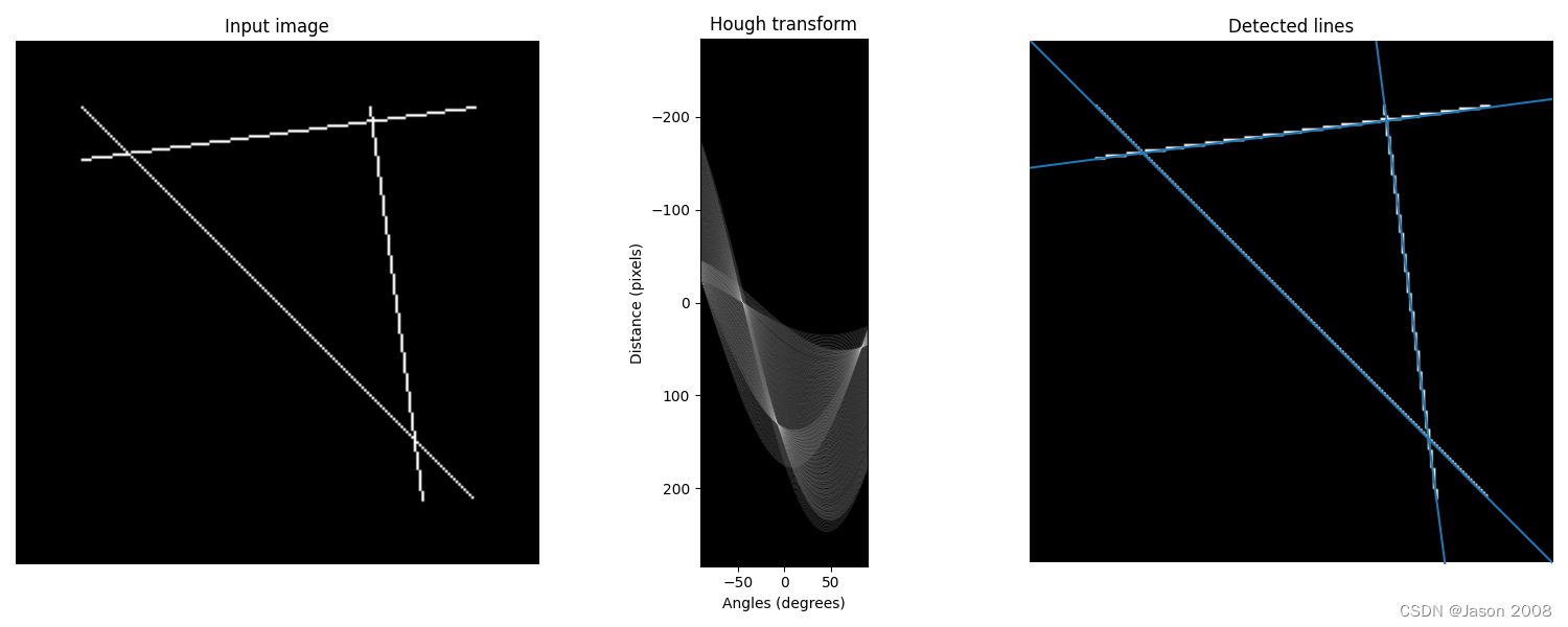
（1）直线检测

使用skimage.transform.hough_line()和skimage.transform.hough_line_peaks()实现直线检测：

skimage.transform.hough_line(image, theta).
skimage.transform.hough_line_peaks(hspace, angles, dists, min_distance, min_angle, threshold, num_peaks)

部分参数说明：

• image：输入图像。
• theta：Angles at which to compute the transform, in radians. Defaults to a vector of 180 angles evenly spaced in the range [-pi/2, pi/2).。
• hspace：Hough transform accumulator。Angles at which the transform is computed, in radians.
• angles：Angles at which the transform is computed, in radians。
• dists：输入图像。
• min_distance：输入图像。
• min_angle：输入图像。
• num_peaks：输入图像。
• hspace：输入图像。

返回值：

• hspace：ndarray of uint64, shape (P, Q)，Hough transform accumulator.
• angles：Angles at which the transform is computed, in radians。

以下是官方提供的一个直线检测的实例：

import numpy as npfrom skimage.transform import hough_line, hough_line_peaks
from skimage.feature import canny
from skimage.draw import line as draw_line
from skimage import dataimport matplotlib.pyplot as plt
from matplotlib import cm# Constructing test image
image = np.zeros((200, 200))
idx = np.arange(25, 175)
image[idx, idx] = 255
image[draw_line(45, 25, 25, 175)] = 255
image[draw_line(25, 135, 175, 155)] = 255# Classic straight-line Hough transform
# Set a precision of 0.5 degree.
tested_angles = np.linspace(-np.pi / 2, np.pi / 2, 360, endpoint=False)
h, theta, d = hough_line(image, theta=tested_angles)# Generating figure 1
fig, axes = plt.subplots(1, 3, figsize=(15, 6))
ax = axes.ravel()ax[0].imshow(image, cmap=cm.gray)
ax[0].set_title('Input image')
ax[0].set_axis_off()angle_step = 0.5 * np.diff(theta).mean()
d_step = 0.5 * np.diff(d).mean()
bounds = [np.rad2deg(theta[0] - angle_step),np.rad2deg(theta[-1] + angle_step),d[-1] + d_step,d[0] - d_step,
]
ax[1].imshow(np.log(1 + h), extent=bounds, cmap=cm.gray, aspect=1 / 1.5)
ax[1].set_title('Hough transform')
ax[1].set_xlabel('Angles (degrees)')
ax[1].set_ylabel('Distance (pixels)')
ax[1].axis('image')ax[2].imshow(image, cmap=cm.gray)
ax[2].set_ylim((image.shape[0], 0))
ax[2].set_axis_off()
ax[2].set_title('Detected lines')for _, angle, dist in zip(*hough_line_peaks(h, theta, d)):(x0, y0) = dist * np.array([np.cos(angle), np.sin(angle)])ax[2].axline((x0, y0), slope=np.tan(angle + np.pi / 2))plt.tight_layout()
plt.show()

以下是处理结果示例：

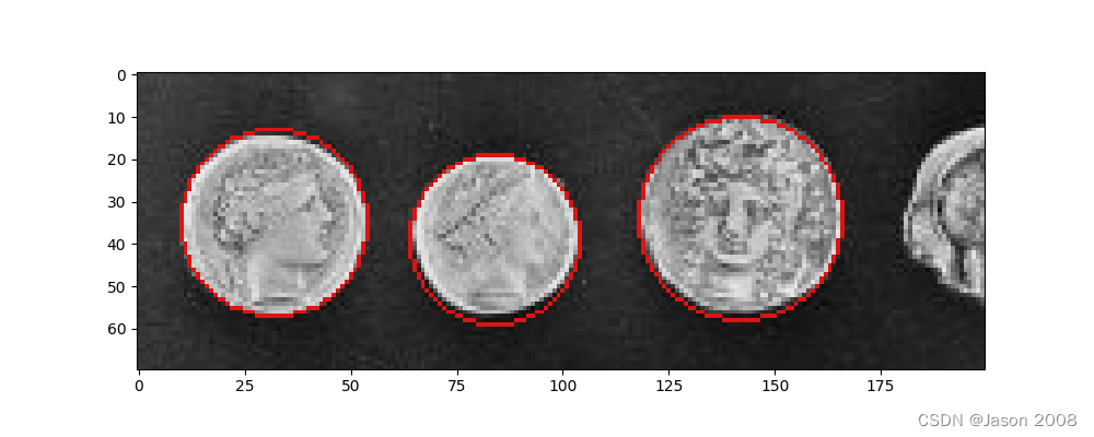
（2）圆形检测

使用skimage.transform.hough_circle()和skimage.transform.hough_circle_peaks()检测圆形：

skimage.transform.hough_circle(image, radius, normalize, full_output)
skimage.transform.hough_circle_peaks(hspaces, radii, min_xdistance, min_ydistance, threshold, num_peaks, total_num_peaks, normalize)

以下是官方提供的一个圆形检测的实例：

import numpy as np
import matplotlib.pyplot as pltfrom skimage import data, color
from skimage.transform import hough_circle, hough_circle_peaks
from skimage.feature import canny
from skimage.draw import circle_perimeter
from skimage.util import img_as_ubyte# Load picture and detect edges
image = img_as_ubyte(data.coins()[160:230, 70:270])
edges = canny(image, sigma=3, low_threshold=10, high_threshold=50)# Detect two radii
hough_radii = np.arange(20, 35, 2)
hough_res = hough_circle(edges, hough_radii)# Select the most prominent 3 circles
accums, cx, cy, radii = hough_circle_peaks(hough_res, hough_radii, total_num_peaks=3)# Draw them
fig, ax = plt.subplots(ncols=1, nrows=1, figsize=(10, 4))
image = color.gray2rgb(image)
for center_y, center_x, radius in zip(cy, cx, radii):circy, circx = circle_perimeter(center_y, center_x, radius, shape=image.shape)image[circy, circx] = (220, 20, 20)ax.imshow(image, cmap=plt.cm.gray)
plt.show()

以下是处理结果示例：

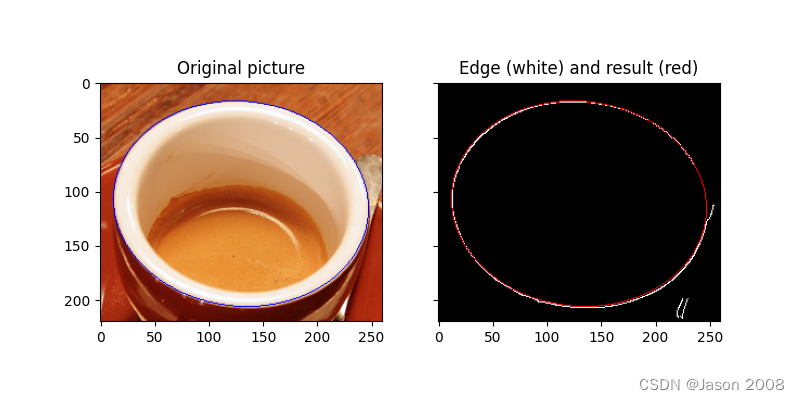
（3）椭圆检测

使用skimage.transform.hough_ellipse()检测椭圆形：

skimage.transform.hough_ellipse(image, threshold, accuracy, min_size, max_size)

以下是官方提供的一个椭圆检测的实例：

import matplotlib.pyplot as pltfrom skimage import data, color, img_as_ubyte
from skimage.feature import canny
from skimage.transform import hough_ellipse
from skimage.draw import ellipse_perimeter# Load picture, convert to grayscale and detect edges
image_rgb = data.coffee()[0:220, 160:420]
image_gray = color.rgb2gray(image_rgb)
edges = canny(image_gray, sigma=2.0, low_threshold=0.55, high_threshold=0.8)# Perform a Hough Transform
result = hough_ellipse(edges, accuracy=20, threshold=250, min_size=100, max_size=120)
result.sort(order='accumulator')# Estimated parameters for the ellipse
best = list(result[-1])
yc, xc, a, b = (int(round(x)) for x in best[1:5])
orientation = best[5]# Draw the ellipse on the original image
cy, cx = ellipse_perimeter(yc, xc, a, b, orientation)
image_rgb[cy, cx] = (0, 0, 255)
# Draw the edge (white) and the resulting ellipse (red)
edges = color.gray2rgb(img_as_ubyte(edges))
edges[cy, cx] = (250, 0, 0)fig2, (ax1, ax2) = plt.subplots(ncols=2, nrows=1, figsize=(8, 4), sharex=True, sharey=True
)ax1.set_title('Original picture')
ax1.imshow(image_rgb)ax2.set_title('Edge (white) and result (red)')
ax2.imshow(edges)plt.show()

以下是处理结果示例：

参考文献：

1. Duda, R. O. and P. E. Hart, “Use of the Hough Transformation to Detect Lines and Curves in Pictures,” Comm. ACM, Vol. 15, pp. 11-15 (January, 1972)
2. C. Galamhos, J. Matas and J. Kittler,”Progressive probabilistic Hough transform for line detection”, in IEEE Computer Society Conference on Computer Vision and Pattern Recognition, 1999.

（未完待续）

这篇关于用Skimage学习数字图像处理（021）：图像特征提取之线检测（下）的文章就介绍到这儿，希望我们推荐的文章对编程师们有所帮助！

---