本文主要是介绍R语言课程论文-飞机失事数据可视化分析,希望对大家解决编程问题提供一定的参考价值,需要的开发者们随着小编来一起学习吧!
数据来源:Airplane Crashes Since 1908 (kaggle.com)
代码参考:Exploring historic Air Plane crash data | Kaggle
| 指标名 | 含义 |
| Date | 事故发生日期(年-月-日) |
| Time | 当地时间,24小时制,格式为hh:mm |
| Location | 事故发生的地点 |
| Operator | 航空公司或飞机的运营商 |
| Flight | 由飞机操作员指定的航班号 |
| Route | 事故前飞行的全部或部分航线 |
| Type | 飞机类型 |
| Registration | 国际民航组织对飞机的登记 |
| cn/In | 结构号或序列号/线号或机身号 |
| Aboard | 机上人数 |
| Fatalities | 死亡人数 |
| Ground | 地面死亡人数 |
| Summary | 事故的简要描述和原 |
library(tidyverse)
library(lubridate)
library(plotly)
library(gridExtra)
library(usmap)
library(igraph)
library(tidytext)
library(tm)
library(SnowballC)
library(wordcloud)
library(RColorBrewer)
library(readxl)df<- read.csv('F:\\Airplane_Crashes_and_Fatalities_Since_1908.csv',stringsAsFactors = FALSE)
df <- as_tibble(df)
head(df)
dim(df)
colnames(df)
df[is.na(df)] <- 0
df$Date <- mdy(df$Date)
df$Time <- hm(df$Time)
df$Year <- year(df$Date)
df$Month <- as.factor(month(df$Date))
df$Day <- as.factor(day(df$Date))
df$Weekday <- as.factor(wday(df$Date))
df$Week_no <- as.factor(week(df$Date))
df$Quarter <- as.factor(quarter(df$Date))
df$Is_Leap_Year <- leap_year(df$Date)
df$Decade <- year(floor_date(df$Date, years(10)))
df$Hour <- as.integer(hour(df$Time))
df$Minute <- as.factor(minute(df$Time))
df$AM_PM <- if_else(am(df$Time), 'AM', 'PM')
df$btwn_6PM_6AM <- if_else(df$Hour <= 6 | df$Hour >= 18, '6PM-6AM', '6AM-6PM')
year_wise <- df %>% count(Year)
day_wise <- df %>% count(Day)
week_day_wise <- df %>% count(Weekday)
month_wise <- df %>% count(Month)
week_no_wise <- df %>% count(Week_no)
q_wise <- df %>% count(Quarter)
hour_wise <- df %>% count(Hour)
am_pm_wise <- df %>% count(AM_PM)
btwn_6PM_6AM_wise <- df %>% count(btwn_6PM_6AM)
Fatalities_wise <- df %>% count(Fatalities)
#图1:自1980年来每年失事飞机失事次数柱状图
ggplot(year_wise, aes(x = Year, y = n)) +geom_col(fill = '#0f4c75', col = 'white') +labs(title = '自1908年以来每年发生的飞机失事次数', x = '', y = '') +scale_x_continuous(breaks = seq(1908, 2020, 4))
#图2:失事飞机失事次数柱状图(按一周第几天、一月第几天统计)
wd <- ggplot(week_day_wise, aes(x = Weekday, y = n)) +geom_col(fill = '#3b6978', col = 'white')+labs(title = '按周的每一天统计飞机失事次', x = '', y = '')
d <- ggplot(day_wise, aes(x = Day, y = n)) +geom_col(fill = '#b83b5e', col = 'white')+labs(title = '按月的每一天统计飞机失事次', x = '', y = '')
grid.arrange(wd, d, nrow = 1, widths = c(1, 3))
#图3:失事飞机失事次数柱状图(按一年第几月、第几周、第几季度统计)
m <- ggplot(month_wise, aes(x = Month, y = n)) +geom_col(fill = '#ffcb74', col = 'white') +labs(title = '按月统计', x = '', y = '')
wn <- ggplot(week_no_wise, aes(x = Week_no, y = n)) +geom_col(fill = '#4f8a8b', col = 'white') +labs(title = '按周统计', x = '', y = '')
q <- ggplot(q_wise, aes(x = Quarter, y = n)) +geom_col(fill = '#ea907a', col = 'white') +labs(title = '按季度统计', x = '', y = '')
grid.arrange(m, wn, q, nrow = 1, widths = c(2, 5, 1))
#图4:失事飞机失事次数柱状图(按一天第几小时、一天中上下午度统计)
h <- ggplot(hour_wise, aes(x = Hour, y = n)) +geom_col(fill = '#BD956A') +labs(title = '按小时统计', x = '', y = '')
a <- ggplot(am_pm_wise, aes(x = AM_PM, y = n, fill = AM_PM)) +geom_col() + labs(title = '上午-下午', x = '', y = '') +scale_fill_brewer(palette = "Set1") +theme(legend.position = "none")
n <- ggplot(btwn_6PM_6AM_wise, aes(x = btwn_6PM_6AM, y = n, fill = btwn_6PM_6AM)) +geom_col() +labs(title = '白天&夜间', x = '', y = '') +scale_fill_brewer(palette = "Dark2") + theme(legend.position = "none")
grid.arrange(h, a, n, nrow = 1, layout_matrix = rbind(c(1,1,1,1,2),c(1,1,1,1,3)))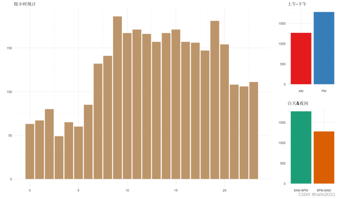
#图5:失事飞机型号统计条形图
# 按类型分组
type_wise <- df %>%count(Type, sort = TRUE)
#按制造商提取和分组
main_type_wise <- df %>%#用空字符串替换型号mutate(main_type = str_replace_all(Type, "[A-Za-z]*-?\\d+-?[A-Za-z]*.*", "")) %>% count(main_type, sort = TRUE) %>%# 跳过空字符串行filter(main_type > 'A')
options(repr.plot.width = 12)
# 失事飞机的型号排名(前20)
ggplot(head(type_wise, 20), aes(reorder(Type, n) , n, fill = n)) +geom_col(fill = 'deepskyblue2') +  geom_text(aes(label = n), hjust = 1.5, colour = "white", size = 5, fontface = "bold") +labs(title = '失事飞机的型号统计', x = '', y = '') +coord_flip()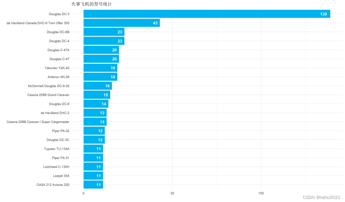
#图6:失事飞机制造商统计条形图
ggplot(head(main_type_wise, 10), aes(reorder(main_type, n), n, fill = n)) +geom_col(fill = 'deepskyblue2') +geom_text(aes(label = n), hjust = 1.5, colour = "white", size = 5, fontface = "bold") +labs(title = '失事飞机的制造商统计', x = '', y = '')+    coord_flip()
#图7:失事飞机(包括军事飞机)运营商统计条形图
#运营商统计
operator_wise <- df %>%count(Operator, sort = TRUE)
#商业运营商表
main_op_wise <- df %>%# replace all group of words followed by '-'mutate(main_op = str_replace_all(Operator, ' -.*', '')) %>% filter(!str_detect(main_op, '[Mm]ilitary')) %>%filter(!str_detect(main_op, 'Private')) %>%count(main_op, sort = TRUE) %>%filter(main_op > 'A')
# 提取军事飞行数据
force <- operator_wise %>%filter(str_detect(Operator, '[Mm]ilitary')) %>%mutate(op = str_replace_all(Operator, 'Military ?-? ?', '')) %>%count(op, sort = TRUE)
#提取军事飞机所属国家
force_country <- operator_wise %>%# 获取包含字符串“军用”的行'military'filter(str_detect(Operator, 'Military|military')) %>%# 将带有包含国家信息的字符串替换为国家名mutate(op = str_replace_all(Operator, 'Royal Air Force', 'UK')) %>%mutate(op = str_replace_all(op, 'Military ?-? ?|Royal', '')) %>%mutate(op = str_replace_all(op, ' (Navy|Army|Air|Maritime Self Defense|Marine Corps|Naval|Defence|Armed) ?.*', '')) %>%mutate(op = str_replace_all(op, '.*U\\.? ?S\\.?.*|United States|American', 'USA')) %>%mutate(op = str_replace_all(op, 'Aeroflot ?/? ?', '')) %>%mutate(op = str_replace_all(op, '.*Republic? ?of', '')) %>%mutate(op = str_replace_all(op, '.*British.*', 'UK')) %>%mutate(op = str_replace_all(op, '.*Indian.*', 'Indian')) %>%mutate(op = str_replace_all(op, '.*Chin.*', 'Chinese')) %>%mutate(op = str_replace_all(op, '.*Chilean.*', 'Chilian')) %>%mutate(op = str_replace_all(op, '.*Iran.*', 'Iran')) %>%mutate(op = str_replace_all(op, '.*French.*', 'French')) %>%mutate(op = str_replace_all(op, '.*Ecuador.*', 'Ecuadorean')) %>%mutate(op = str_replace_all(op, '.*Zambia.*', 'Zambian')) %>%mutate(op = str_replace_all(op, '.*Russia.*', 'Russian')) %>%mutate(op = str_replace_all(op, '.*Afghan.*', 'Afghan')) %>%group_by(op) %>%summarize(n = sum(n)) %>%arrange(desc(n))
#军用飞行与非军用飞行
yr_military <- df %>%select(Year, Operator) %>%mutate(Is_Military = str_detect(Operator, 'Military|military')) %>%group_by(Year, Is_Military) %>%summarize(n = n())
ggplot(head(operator_wise, 10), aes(reorder(Operator, n) , n, fill = n))+geom_col(fill = 'coral3')+labs(title='失事飞机(包括军事飞机在内)的运营商统计', x = '', y = '')+  geom_text(aes(label = n), hjust = 1.5, colour = "white", size = 5, fontface = "bold")+coord_flip()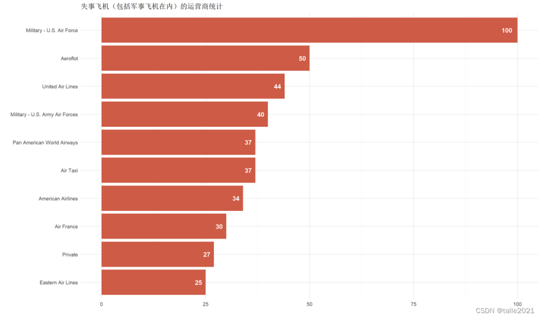
#图8:失事飞机(不包括军事飞机)运营商统计条形图
ggplot(head(main_op_wise, 10), aes(reorder(main_op, n) , n, fill=n)) +geom_col(fill='coral2') +labs(title='失事商业飞机(不包括军事飞机)的商业运营商统计', x='', y='') +  geom_text(aes(label = n), hjust = 1.5, colour = "white", size = 5, fontface = "bold") +coord_flip()
#图9:军事飞机所属军队、所属国家统计条形图
f <- ggplot(head(force, 10), aes(reorder(op, n) , n, fill = n))+geom_col(fill = 'cyan4')+labs(title = '军事飞机失事统计', x = '', y = '')+  geom_text(aes(label = n), hjust = 1.5, colour = "white", size = 5, fontface = "bold")+coord_flip()
fc <- ggplot(head(force_country, 10), aes(reorder(op, n) , n, fill = n))+geom_col(fill = 'cyan3')+labs(title = '军事飞机失事的国家排名', x = '', y = '')+  geom_text(aes(label = n), hjust = 1.5, colour = "white", size = 5, fontface = "bold")+coord_flip()
grid.arrange(f,fc, nrow = 1, widths = c(1, 1))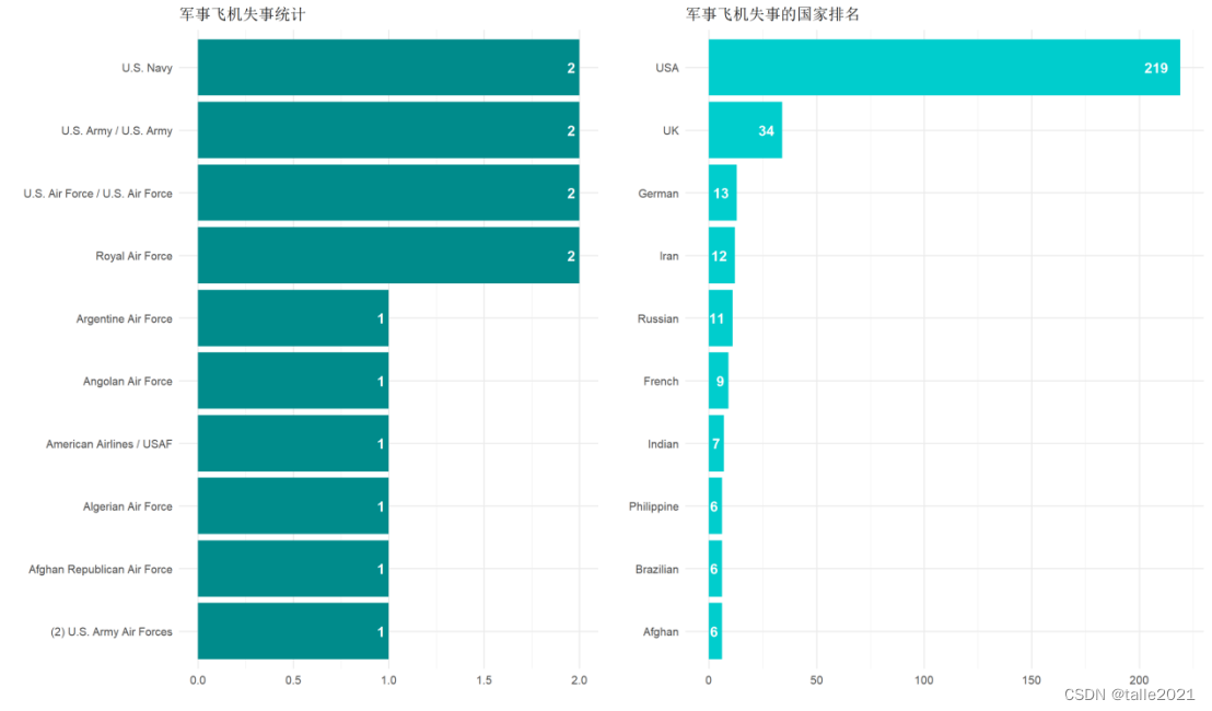
#图10:自1980年来军事飞机与非军事失事次数柱状图
ggplot(yr_military, aes(x = Year, y = n, fill = Is_Military)) +geom_col(col = 'white') +labs(title = '失事飞机是否为军用飞机?',x = '', y = '', fill = '') +scale_x_continuous(breaks = seq(1908, 2020, 4)) + scale_fill_brewer(palette = "Dark2") +theme(legend.position = "top", legend.justification = "left")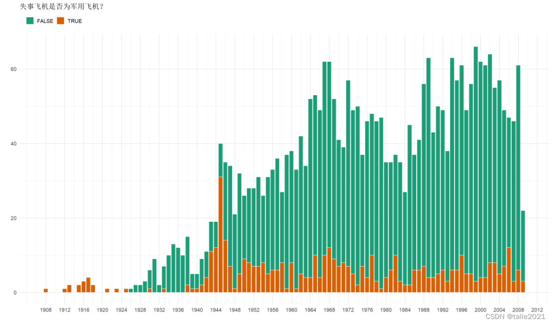
#图11:飞机失事地点统计条形图
take_off_dest <- df %>%select('Route') %>%filter(Route!='') %>%filter(str_detect(Route, ' ?- ?')) %>%mutate(Take_Off = str_extract(Route, '[^-]* ?-?')) %>%mutate(Take_Off = str_replace(Take_Off, ' -', ''))%>%mutate(Destination = str_extract(Route, '- ?[^-]*$')) %>%mutate(Destination = str_replace(Destination, '- ?', ''))
route <- take_off_dest %>% count(Route, sort = TRUE)
take_off <- take_off_dest %>% count(Take_Off, sort = TRUE)
dest <- take_off_dest %>% count(Destination, sort = TRUE)
r <- ggplot(head(route, 15), aes(reorder(Route, n) , n, fill=n))+geom_col(fill='#E59CC4')+labs(title='飞行途中失事路线', x='', y='')+  geom_text(aes(label=n), hjust = 1.5, colour="white", size=5, fontface="bold")+coord_flip()
t <- ggplot(head(take_off, 15), aes(reorder(Take_Off, n) , n, fill=n))+geom_col(fill='#005082')+labs(title='起飞时飞机失事地点', x='', y='')+  geom_text(aes(label=n), hjust = 1.5, colour="white", size=5, fontface="bold")+coord_flip()
d <- ggplot(head(dest, 15), aes(reorder(Destination, n) , n, fill=n))+geom_col(fill='#ff6363')+labs(title='落地时飞机失事地点', x='', y='')+  geom_text(aes(label=n), hjust = 1.5, colour="white", size=5, fontface="bold")+coord_flip()
options(repr.plot.width = 18)
grid.arrange(r,t,d, nrow = 1, widths=c(1,1,1))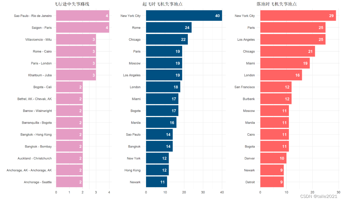
#图12:全球范围内飞机失事热力图
cntry <- cntry %>%mutate(m = case_when(n >= 100  ~ "100 +",n < 100 & n >= 70 ~ "70 - 100",n < 70 & n >= 40 ~ "40 - 70",n < 40 & n >= 10 ~ "10 - 40",n < 10  ~ "< 10")) %>%mutate(m = factor(m, levels = c("< 10", "10 - 40", "40 - 70", "70 - 100", "100 +")))
world_map <- map_data("world")
map_data <- cntry %>% full_join(world_map, by = c('Country' = 'region'))
options(repr.plot.width = 18, repr.plot.height = 9)
map_pal = c("#7FC7AF", "#E4B363",'#EF6461',"#E97F02",'#313638')
ggplot(map_data, aes(x = long, y = lat, group = group, fill = m)) +geom_polygon(colour = "white") + labs(title = '全球范围内飞机失事热力图', x = '', y = '', fill = '') +scale_fill_manual(values = map_pal, na.value = 'whitesmoke') + theme(legend.position='right', legend.justification = "top") + guides(fill = guide_legend(reverse = TRUE))
#图13:飞机失事原因词云图
data <- read_excel("F:\\summary.xlsx")
corpus <- Corpus(VectorSource(data))
corpus <- tm_map(corpus, content_transformer(tolower))
corpus <- tm_map(corpus, removePunctuation)
corpus <- tm_map(corpus, removeNumbers)
corpus <- tm_map(corpus, removeWords, stopwords("english"))dtm <- TermDocumentMatrix(corpus)
word_freqs <- rowSums(as.matrix(dtm))
wordcloud(names(word_freqs), word_freqs, min.freq = 1, max.words=150,words_distance=0.001,random.order=FALSE,font_path='msyh.ttc',
rot.per=0.05,colors=brewer.pal(8, "Dark2"), backgroundColor = "grey",shape = 'circle',width=3, height=9)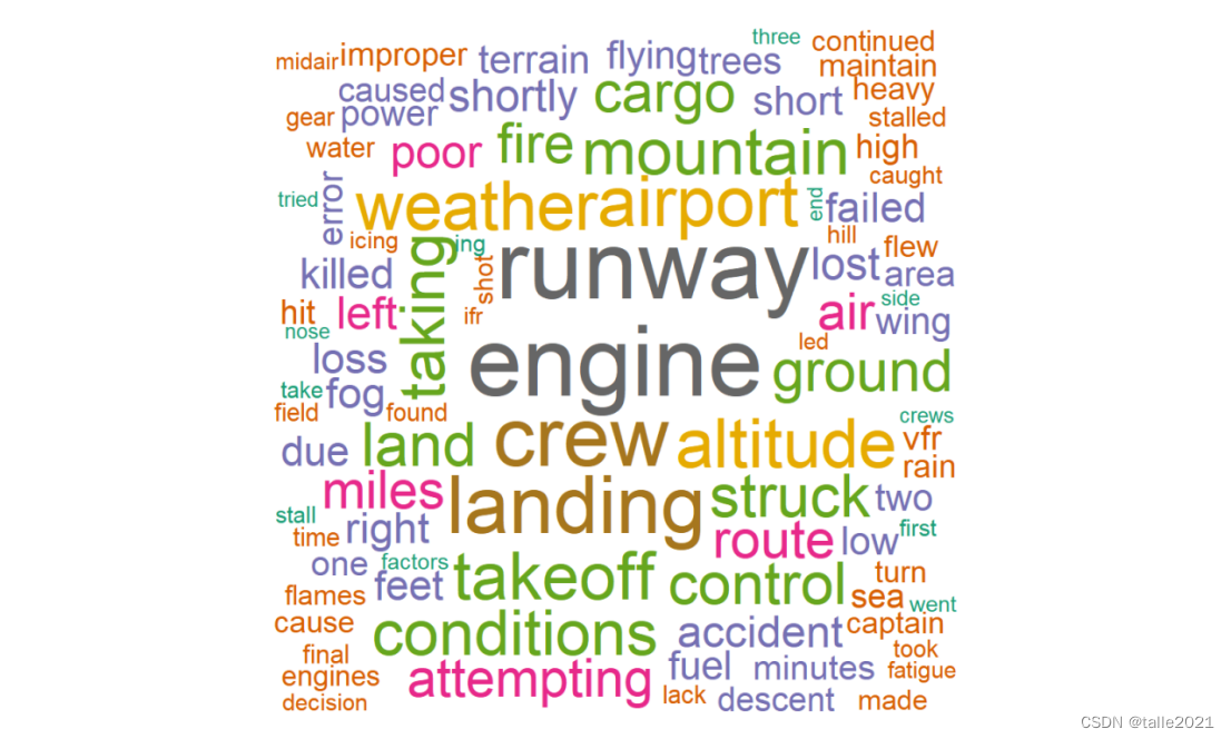
ps:低价出课程论文-多元统计分析论文、R语言论文、stata计量经济学课程论文(论文+源代码+数据集)
这篇关于R语言课程论文-飞机失事数据可视化分析的文章就介绍到这儿,希望我们推荐的文章对编程师们有所帮助!


