cc和毫升换算_新加坡房屋价格毫升预测分析新加坡房地产价格第三部分

In part I of this series on Singapore’s housing prices, I have focused on the extraction of additional information and create new distance-related variables that may have an impact on housing prices. In part II, using data visualisation, I have showed that the proximity of flats to amenities, especially transport, food centres and top schools, have a significant impact on the housing prices.

在一部分我这个系列新加坡的房价，我都集中在附加信息的提取，并创建可能对住房价格产生影响新的距离有关的变量。 在第二部分中 ，我使用数据可视化显示了公寓与便利设施(尤其是交通，食品中心和顶级学校)之间的距离对房价产生了重大影响。

In this final part, I will share some popular machine learning algorithms to predict the housing prices and the live model that I have built. My objective is to find a model that can generate a high accuracy of the housing prices, based on the available dataset, such that given a new property and with the required information, we will know whether the property is over or under-valued.

在最后一部分中，我将分享一些流行的机器学习算法，以预测房价和所构建的实时模型。 我的目标是根据可用的数据集找到一个可以生成高精度住房价格的模型，以便在给定新属性并提供所需信息的情况下，我们将知道该属性是高估还是低估了。

所使用的机器学习算法简介 (Brief introduction of the machine learning algorithms used)

I explore 5 machine learning algorithms that are used to predict the housing prices in Singapore, namely multi-linear regression, lasso, ridge, decision tree and neural network.

我探索了5种用于预测新加坡房价的机器学习算法，即多元线性回归，套索，岭，决策树和神经网络。

Multi-linear regression model, as its name suggest, is a widely used model that assumes linearity between the independent variables and dependent variable (price). This will be my baseline model for comparison.

顾名思义，多线性回归模型是一种广泛使用的模型，它假设自变量与因变量(价格)之间呈线性关系。 这将是我的比较基准模型。

Lasso and ridge are models to reduce model complexity and overfitting when there are too many parameters. For example, the lasso model will effectively shrink some of the variables, such that it only takes into account some of the important factors. While there are only 17 variables, in the dataset and the number of variables may not be considered extensive, it will still be a good exercise to analyse the effectiveness of these models.

套索和山脊是用于减少参数过多时模型复杂性和过度拟合的模型。 例如，套索模型将有效地缩小某些变量，从而仅考虑一些重要因素。 尽管只有17个变量，但是在数据集中，变量的数量可能不算是广泛的，分析这些模型的有效性仍然是一个很好的练习。

Decision tree is an easily understandable model which uses a set of binary rules to achieve the target value. This is extremely useful for decision making as a tree diagram can be plotted to aid in understanding the importance of each variable (the higher the variable in the tree, the more important the variable).

决策树是一种易于理解的模型，它使用一组二进制规则来实现目标值。 这对于决策非常有用，因为可以绘制树形图以帮助理解每个变量的重要性(树中的变量越高，变量越重要)。

Last, I have also explored a simple multi-layer perceptron neural network model. Simply put, the data inputs is put through a few layers of “filters” (feed forward hidden layers) and the model learns how to minimise the loss function by changing the values in the “filters” matrices.

最后，我还探索了一个简单的多层感知器神经网络模型。 简而言之，数据输入经过几层“过滤器”(前馈隐藏层)，模型学习如何通过更改“过滤器”矩阵中的值来最小化损失函数。

数据集概述 (Dataset overview)

There are 17 independent variables that are obtained from the dataset, with almost 1/3 of the variables linked to the characteristic of the flat, such as floor area, location, years of lease left etc. The other variables are related to distances of the flat to amenities as well as the neighbourhood’s crime rates.

从数据集中可以获得17个独立变量，其中几乎1/3的变量与公寓的特征有关，例如建筑面积，位置，剩余租赁年限等。其他变量与建筑的距离有关。与便利设施以及邻里的犯罪率持平。

# If we only use the HDB's information without new distance information
df_final = df[['resale_price', 'floor_area_sqm', 'est_floor', 'LATITUDE', 'LONGITUDE', 'total_dwelling_units', 'flat_remainlease']]# If we only use the HDB's information AND new distance information
df_final = df[['resale_price', 'floor_area_sqm', 'est_floor', 'LATITUDE', 'LONGITUDE', 'total_dwelling_units', 'flat_remainlease', 'distance_sch', 'distance_mrt', 'distance_supermarket', 'distance_hawker', 'distance_city', 'distance_npc', 'housebreaking', 'outrage_of_modesty', 'robbery', 'snatch_theft', 'theft_mv']]

数据集探索性聚类可视化 (Dataset exploratory clustering visualisation)

Instead of running numerous pairplots correlation graph, I use the T-distributed Stochastic Neighbor Embedding (t-SNE), a machine learning algorithm to further visualise the correlation between the independent variables and housing prices. t-SNE reduces the high-dimensional data into a low two-dimensional space. The 17 independent variables are reduced to x-y coordinates and the colour of each data point represent the price of the flat. The clustering of data points by flat prices is clearly evident in the image below. Therefore, if we run regression algorithms, we should obtain highly accurate predictive models.

我没有运行大量的成对图相关图，而是使用T分布随机邻居嵌入(t-SNE)，这是一种机器学习算法，可以进一步可视化自变量与房价之间的相关性。 t-SNE将高维数据缩减为低二维空间。 17个独立变量被简化为xy坐标，每个数据点的颜色代表该公寓的价格。 下图清楚显示了按固定价格对数据点进行的聚类。 因此，如果运行回归算法，我们应该获得高度准确的预测模型。

预测模型的数据集准备 (Dataset preparation for predictive modelling)

The train and test dataset are split 80/20 and scaled. Scaling of the independent variables (X_train, X_test) is essential, both for model convergence and speed. If we do not scale large feature values, optimisation functions may not converge as data may swings widely and the large data points will also dominate the learning process, leading to model inaccuracy.

训练和测试数据集被拆分为80/20并缩放。 自变量(X_train，X_test)的缩放对于模型收敛和速度都至关重要。 如果我们不按比例缩放大特征值，那么优化函数可能不会收敛，因为数据可能会大幅波动，大数据点也将主导学习过程，从而导致模型不准确。

import numpy as np
from sklearn.model_selection import train_test_split
from sklearn.preprocessing import StandardScaler# split data into train and test
resale_p = df_final['resale_price'].values
X = df_final.drop(['resale_price'], axis = 1).valuesX_train, X_test, y_train, y_test = train_test_split(X, resale_p, test_size=0.2, random_state=42)# scale the data
scaler = StandardScaler()# the use of fit is to find the mean and variance
X_train = scaler.fit_transform(X_train)# For the test dataset, you do not need to use fit again, as we are using the mean and variance from the train dataset
X_test = scaler.transform(X_test)

机器学习算法 (Machine Learning algorithms)

Sklearn is a popular library package that provides easy accessibility and application of different machine learning algorithms. I have shared the codes below to show the ease of applying various algorithms using the sklearn library package, as they are of similar code syntax.

Sklearn是一个受欢迎的库程序包，可轻松访问和应用各种机器学习算法。 我共享了以下代码，以展示使用sklearn库软件包应用各种算法的简便性，因为它们具有相似的代码语法。

In addition, I have used tensorflow to build a multi-layer perceptron neural network. Due to the relatively small size of the dataset, it does not cause any computational inefficiency when running 500 epoches with batch size of 128. I have attempted to use fewer number of neurons in each hidden layer and the convergence on the training loss is much slower.

另外，我已经使用张量流来构建多层感知器神经网络。 由于数据集的大小相对较小，当运行500个批处理量为128的epoch时，它不会引起任何计算效率低下。我尝试在每个隐藏层中使用较少数量的神经元，并且训练损失的收敛速度慢得多。

from sklearn.linear_model import LinearRegression
from sklearn.linear_model import Lasso
from sklearn.linear_model import Ridge
from sklearn.tree import DecisionTreeRegressorimport tensorflow as tf
from tensorflow import keras
from keras import layers, optimizersdef linreg(X_train, y_train, X_test, y_test):model_results = {}model = LinearRegression()model.fit(X_train, y_train)y_pred = model.predict(X_test)model_results['model'] = 'Linear Regression'model_results['mae'] = metrics.mean_absolute_error(y_test, y_pred)model_results['mse'] = metrics.mean_squared_error(y_test, y_pred)model_results['accuracy'] = metrics.explained_variance_score(y_test, y_pred)return model_resultsdef lasso(X_train, y_train, X_test, y_test):model_results = {}model = Lasso(alpha=1.0)model.fit(X_train, y_train)y_pred = model.predict(X_test)model_results['model'] = 'Lasso'model_results['mae'] = metrics.mean_absolute_error(y_test, y_pred)model_results['mse'] = metrics.mean_squared_error(y_test, y_pred)model_results['accuracy'] = metrics.explained_variance_score(y_test, y_pred)return model_resultsdef ridge(X_train, y_train, X_test, y_test):model_results = {}model = Ridge()model.fit(X_train, y_train)y_pred = model.predict(X_test)model_results['model'] = 'Ridge'model_results['mae'] = metrics.mean_absolute_error(y_test, y_pred)model_results['mse'] = metrics.mean_squared_error(y_test, y_pred)model_results['accuracy'] = metrics.explained_variance_score(y_test, y_pred)return model_resultsdef decisiontree(X_train, y_train, X_test, y_test):model_results = {}model = DecisionTreeRegressor()model.fit(X_train, y_train)y_pred = model.predict(X_test)model_results['model'] = 'Decision Tree'model_results['mae'] = metrics.mean_absolute_error(y_test, y_pred)model_results['mse'] = metrics.mean_squared_error(y_test, y_pred)model_results['accuracy'] = metrics.explained_variance_score(y_test, y_pred)return model_resultsdef nn(X_train, X_test, y_train, y_test, batchsize = 128, training_epochs = 500):tf.keras.backend.clear_session()model_results = {}model = tf.keras.Sequential()model.add(tf.keras.layers.Dense(50, activation = 'relu'))model.add(tf.keras.layers.Dense(50, activation = 'relu'))model.add(tf.keras.layers.Dense(50, activation = 'relu'))model.add(tf.keras.layers.Dense(1))model.compile(optimizer = 'Adam', loss = 'mse')model.fit(x=X_train, y=y_train,validation_data=(X_test,y_test), shuffle = True,batch_size= batchsize, epochs = training_epochs, verbose = 0)y_pred = model.predict(X_test)model_results['model'] = 'Neural Network'model_results['mae'] = metrics.mean_absolute_error(y_test, y_pred)model_results['mse'] = metrics.mean_squared_error(y_test, y_pred)model_results['accuracy'] = metrics.explained_variance_score(y_test, y_pred)return model_resultsmodel_lr = lr(X_train, y_train, X_test, y_test)
model_lasso = lasso(X_train, y_train, X_test, y_test)
model_ridge = ridge(X_train, y_train, X_test, y_test)
model_decision = decisiontree(X_train, y_train, X_test, y_test)
model_nn = nn(X_train, X_test, y_train, y_test, batchsize = 128, training_epochs = 500)
df = pd.DataFrame([model_lr, model_lasso, model_ridge, model_decision, model_nn])

结果 (Results)

So we finally come to the exciting bit of this article. Results.

因此，我们终于来到了这篇文章令人兴奋的地方。 结果。

As mentioned above, I have investigated two scenarios, where I only consider the flats’ characteristics only and the other, where I included more variables such as distance from amenities.

如上所述，我研究了两种情况，其中仅考虑公寓的特征，另一种情况包括更多变量，例如与设施的距离。

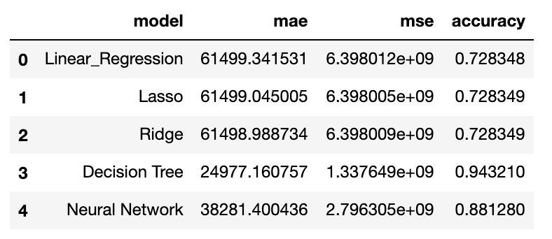
The results show that the additional variables increase model accuracy (using sklearn metrics “explained_variance_score”, similar to R2) by 10% for some of the algorithms. The baseline model (multi-linear regression) accuracy increase from 73% to 84%. This shows the importance of geodistance variables. The results from lasso and ridge do not differ much from the baseline model. For the neural network algorithm, it reports a higher accuracy compared to the baseline model for both scenarios.

结果表明，对于某些算法，附加变量将模型准确性提高了10％(使用sklearn指标“ explained_variance_score”，类似于R2)。 基线模型(多线性回归)的准确性从73％提高到84％。 这表明了地理距离变量的重要性。 套索和山脊的结果与基线模型相差不大。 对于神经网络算法，与两种情况下的基线模型相比，它报告的准确性更高。

The Decision Tree algorithm performs the best in both scenarios. In particular, it achieves a high accuracy rate of 94%, regardless of the additional variables added. The algorithm also reports a Mean Absolute Error (“MAE”) of $24,997, the lowest among the various predictive models. This is relatively low, compared to the cost of a flat. ranging from $150K to $1.2m.

决策树算法在两种情况下均表现最佳。 尤其是，无论添加了其他变量如何，它都能达到94％的高精度。 该算法还报告了24,997美元的平均绝对误差(“ MAE”)，是各种预测模型中最低的。 与公寓的成本相比，这是相对较低的。 从15万美元到120万美元不等。

建立现场模型 (Build a live model)

Going back to the objective of this series of articles on Singapore’s housing prices, the aim is to generate geodistance-based variables, identify if they are of any use in predictive modelling and if so, create a model to help identify whether a house is over or under value.

回到本系列有关新加坡房价的文章的目标，目的是生成基于地理距离的变量，确定它们在预测建模中是否有用，如果有，则创建一个模型以帮助确定房屋是否已过期或低于价值。

Since I have identified distance to amenities as important variables and the Decision Tree algorithm has the highest accuracy amongst the algorithms explored, I then build a live model (using Decision Tree algorithm) based on the findings.

由于我已经确定了到设施的距离是重要的变量，并且决策树算法在所探索的算法中具有最高的准确性，因此我根据发现结果构建了一个实时模型(使用决策树算法)。

# import py files containing codes to find postal address and nearest amenties and distances
import find_postal_address
import Distance_from_amenities# User inputs
flat = input("Enter address: ")
floor_area = input("Floor area in sqm (not sq feet): ")
flat_level = input("Floor Level: ")# Generate user_info_inputs
floor_area = int(floor_area)
flat_level = int(flat_level)
user_input_info = np.array((floor_area, flat_level)).reshape(1, -1)  #<--- user inputs# Generate hdb info inputs
target = [flat]target_clean = []
for i in target:target_clean.append(i.upper().replace('ROAD', 'RD').replace('STREET', 'ST').replace('CENTRAL', 'CTRL'))find_postal_address.find_postal(target_clean, 'target')
geo = pd.read_csv("target.csv")
geo1 = geo[['address', 'LATITUDE', 'LONGITUDE']]df_base = pd.read_csv('hdb-property-information.csv')
df_base = df_base[['blk_no', 'street', 'year_completed', 'total_dwelling_units']]
df_base['address'] = df_base['blk_no'] + " " + df_base['street']
target_base = pd.merge(geo1, df_base, how = 'left', left_on=['address'], right_on=['address'])
target_base['flat_remainlease'] = 2020 - target_base['year_completed']
hdb_info = target_base[['LATITUDE', 'LONGITUDE', 'total_dwelling_units', 'flat_remainlease']].values  #<--- hdb inputs# Generate distance info inputs# For Mrt - # find nearest train station to the flat
mrt = pd.read_excel("mrt_list.xlsx")
mrt1 = mrt[['STN_NAME', 'Latitude', 'Longitude']]
map_mrt = Distance_from_amenities.find_nearest(geo1,mrt1)# For hawkers centres - # find nearest hawker centre to the flat
hawker = pd.read_csv('hawker_geoloc_new.csv')
hawker1 = hawker[['address', 'LATITUDE', 'LONGITUDE']]
map_hawker = Distance_from_amenities.find_nearest(geo1,hawker1)# For school - # find nearest school to the flat
sch = pd.read_csv('school_geoloc.csv')
sch1 = sch[['address', 'LATITUDE', 'LONGITUDE']]
map_prisch = Distance_from_amenities.find_nearest(geo1,sch1)# For supermarkets - # find nearest supermarket to the flat
supermarket = pd.read_csv('supermarket_geoloc.csv')
supermarket1 = supermarket[['ADDRESS', 'LATITUDE', 'LONGITUDE']]
map_supermarket = Distance_from_amenities.find_nearest(geo1,supermarket1)# For neighborhood police centre - # find nearest police station to the flat
crimes = pd.read_csv('npc_geoloc.csv')
crimes1 = crimes[['address', 'LATITUDE', 'LONGITUDE']]
map_crimes = Distance_from_amenities.find_nearest(geo1,crimes1)# For city centre - # Measure distance from city centre to the flat
data = [['cityhall', 1.29317576, 103.8525073]] 
sgcentre = pd.DataFrame(data, columns = ['address', 'LATITUDE', 'LONGITUDE'])
map_sgcentre = Distance_from_amenities.find_nearest(geo1,sgcentre)columns = ['prisch', 'mrt', 'supermarket', 'hawker', 'city', 'neigbourhood_police_post']
target_df = pd.DataFrame([map_prisch, map_mrt, map_supermarket, map_hawker, map_sgcentre, map_crimes])
address = target_df.columns.tolist()
address = str(address).strip("'[]'")
target_df1 = pd.DataFrame(target_df[address].to_list(), columns = ['address', 'amenity', 'distance'])target_df1['type of amenties'] = columns 
target_df1.drop(['address'], axis = 1)
target_df1 = target_df1[['type of amenties', 'amenity', 'distance']]print('\n')
print(target_df1)
distance_info= target_df1['distance'].astype(str).str[:-2].astype(float).values# crime inputs
crime5 = pd.read_csv("/Users/michaelongwenyun/Desktop/Github/ST445_visualisation/2019mt-st445-project-MichaelWYOng/crime_wide.csv")
npc_name = list(map_crimes.values())[0][1]
crime_info = crime5[crime5['npc'] == npc_name]
crime_info = crime_info.drop(['npc'], axis = 1).values# Put all info together
distance_info = distance_info.reshape(1, -1)
target_np = np.concatenate((user_input_info, hdb_info, distance_info, crime_info), axis = 1).reshape(-1,17)# prediction
target_np = scaler.transform(target_np)
valuation_price = model.predict(target_np)print('\n')
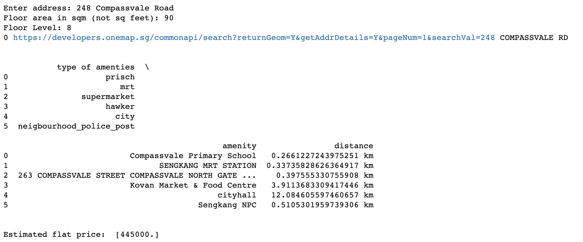
print('Estimated flat price: ', valuation_price)

The user has to input 3 information (“address of the flat”, “floor area of the flat” and “floor level of the flat”). The rest of the variables are extracted from the metadata of public housings and also using the codes in Part I to generate the geodistance variables. Using two latest listing on propertyguru in Sengkang area and assuming they are on floor level 8 (the floor level is not indicated in the property listings), it is noted that one property is selling below the predicted value while the other is selling at the predicted value. This can help buyers identify whether they are getting a fair value for a flat that they are interested in; and also help sellers to identify whether they have set a reasonable listing price for their flats.

用户必须输入3个信息(“公寓的地址”，“公寓的地板面积”和“公寓的地板高度”)。 其余变量是从公共住房的元数据中提取的，并且还使用第一部分中的代码来生成地理距离变量。 使用Sengkang地区最新的两个房地产专家清单，并假设它们位于第8层(该房地产清单中未列出该层)，请注意，一处物业的售价低于预期，而另一处物业的售价低于预期。值。 这可以帮助买家确定他们是否对感兴趣​​的公寓获得了公允价值； 并帮助卖家确定他们是否为单位设定了合理的挂牌价格。

结论 (Conclusion)

In this last part of the series on Singapore’s housing prices, I have investigate various machine learning algorithms to predict housing prices and conclude that the Decision Tree algorithm (out of the 5 models explored) has the highest accuracy. Furthermore, I build a live model such that it can take any new flat listing, generate a predicted value of the flat and be compared with the listing price of a property. This will give an indication of whether the listed flat is a “good buy”.

在有关新加坡住房价格的系列的最后一部分中，我研究了各种机器学习算法来预测住房价格，并得出结论：决策树算法(在所研究的5种模型中)具有最高的准确性。 此外，我建立了一个实时模型，使它可以接受任何新的公寓上市，生成该公寓的预测价值，并与房地产的挂牌价进行比较。 这将表明上市公寓是否是“好买”。

The accuracy of the model can be further improved, such as taking into consideration other time series variables, i.e. macroeconomic variables. Also, cross validation is always a good practice to ensure consistency of model. Nevertheless, with the high accuracy rate obtained from this model, it should suffice for this study.

可以进一步提高模型的准确性，例如考虑其他时间序列变量，即宏观经济变量。 此外，交叉验证始终是确保模型一致性的一种良好做法。 然而，由于从该模型获得的高准确率，该研究就足够了。