BikeDNA（二） OSM数据的内在分析1

本文主要是介绍BikeDNA（二） OSM数据的内在分析1，希望对大家解决编程问题提供一定的参考价值，需要的开发者们随着小编来一起学习吧！

BikeDNA（二） OSM数据的内在分析1

该笔记本分析给定区域的 OSM 自行车基础设施数据的质量。 质量评估是“内在的”，即仅基于一个输入数据集，而不使用外部信息。 对于将 OSM 数据与用户提供的参考数据集进行比较的外在质量评估，请参阅笔记本 3a 和 3b。

该分析评估给定区域 OSM 数据的“目的适应性”（Barron et al., 2014）。 分析的结果可能与自行车规划和研究相关 - 特别是对于包括自行车基础设施网络分析的项目，在这种情况下，几何拓扑尤为重要。

由于评估不使用外部参考数据集作为基本事实，因此无法对数据质量做出普遍的声明。 这个想法是让那些使用基于 OSM 的自行车网络的人能够评估数据是否足以满足他们的特定用例。 该分析有助于发现潜在的数据质量问题，但将结果的最终解释权留给用户。

该笔记本利用了一系列先前调查 OSM/VGI 数据质量的项目的质量指标，例如 Ferster et al. (2020), Hochmair et al. (2015), Barron et al. (2014), and Neis et al. (2012)。

该笔记本的输出文件（数据、地图、绘图）保存到…/results/OSM/[study_area]/ subfolders.

# Load libraries, settings and dataimport json
import pickle
import warnings
from collections import Counter
import mathimport contextily as cx
import folium
import geopandas as gpd
import matplotlib as mpl
import matplotlib.patches as mpatches
import matplotlib.pyplot as plt
import numpy as np
import osmnx as ox
import pandas as pd
import yaml
from matplotlib import cm, colorsfrom src import evaluation_functions as eval_func
from src import plotting_functions as plot_func%run ../settings/yaml_variables.py
%run ../settings/plotting.py
%run ../settings/tiledict.py
%run ../settings/load_osmdata.py
%run ../settings/df_styler.py
%run ../settings/paths.pywarnings.filterwarnings("ignore")grid = osm_grid

D:\tmp_resource\BikeDNA-main\BikeDNA-main\scripts\settings\plotting.py:49: MatplotlibDeprecationWarning: The get_cmap function was deprecated in Matplotlib 3.7 and will be removed two minor releases later. Use ``matplotlib.colormaps[name]`` or ``matplotlib.colormaps.get_cmap(obj)`` instead.cmap = cm.get_cmap(cmap_name, n)
D:\tmp_resource\BikeDNA-main\BikeDNA-main\scripts\settings\plotting.py:46: MatplotlibDeprecationWarning: The get_cmap function was deprecated in Matplotlib 3.7 and will be removed two minor releases later. Use ``matplotlib.colormaps[name]`` or ``matplotlib.colormaps.get_cmap(obj)`` instead.cmap = cm.get_cmap(cmap_name)OSM graphs loaded successfully!
OSM data loaded successfully!<string>:49: MatplotlibDeprecationWarning: The get_cmap function was deprecated in Matplotlib 3.7 and will be removed two minor releases later. Use ``matplotlib.colormaps[name]`` or ``matplotlib.colormaps.get_cmap(obj)`` instead.
<string>:46: MatplotlibDeprecationWarning: The get_cmap function was deprecated in Matplotlib 3.7 and will be removed two minor releases later. Use ``matplotlib.colormaps[name]`` or ``matplotlib.colormaps.get_cmap(obj)`` instead.

1.数据完整性

1.1 网络密度

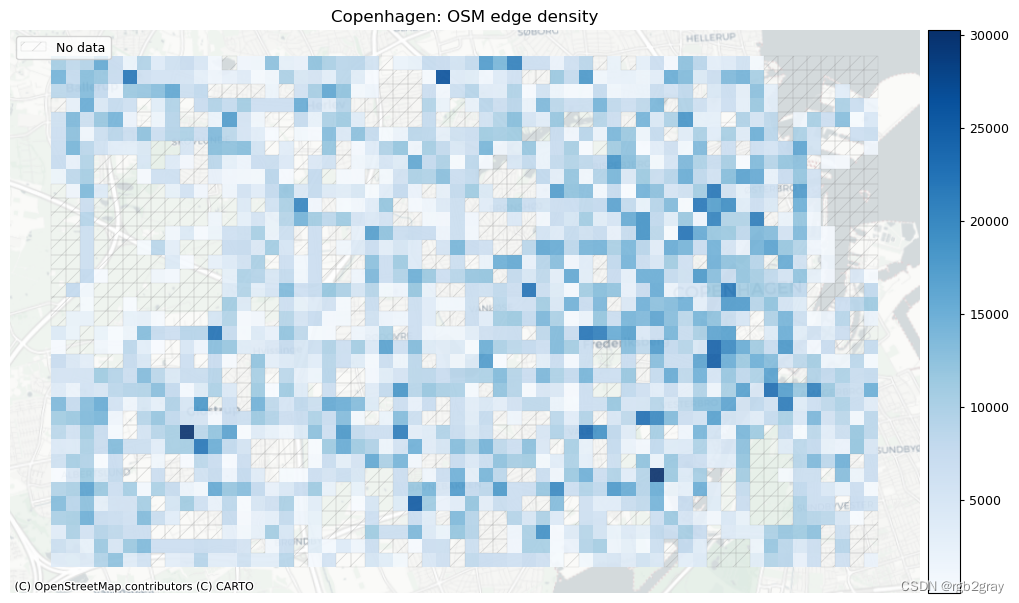
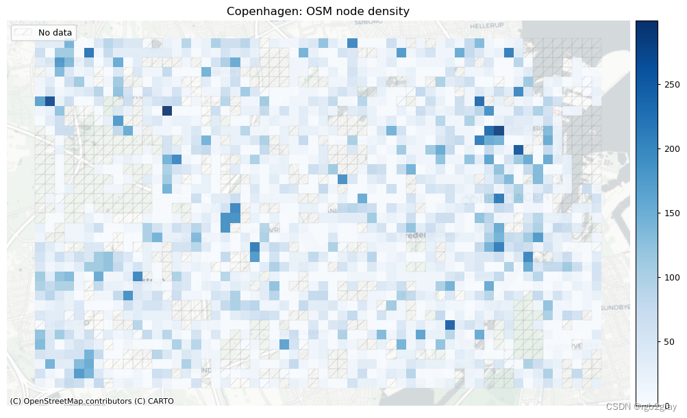
在此设置中，网络密度是指边的长度或每平方公里的节点数。 这是空间（道路）网络中网络密度的通常定义，它与网络科学中更常见的“结构”网络密度不同。 如果不与参考数据集进行比较，网络密度本身并不表明空间数据质量。 然而，对于熟悉研究区域的任何人来说，网络密度可以表明该区域的某些部分是否映射不足或过度。

方法

这里的密度不是基于边缘的几何长度，而是基于基础设施的计算长度。 例如，一条 100 米长的双向路径贡献了 200 米的自行车基础设施。 该方法用于考虑绘制自行车基础设施的不同方式，否则可能会导致网络密度出现较大偏差。 使用“compute_network_densis”，可以计算每单位面积的元素数量（节点、悬空节点和基础设施总长度）。 密度计算两次：首先计算整个网络的研究区域（“全局密度”），然后计算每个网格单元（“局部密度”）。 全局和局部密度都是针对整个网络以及受保护和未受保护的基础设施计算的。

解释

由于此处进行的分析是内在的，即不使用外部信息，因此无法知道低密度值是由于测绘不完整还是由于该地区实际缺乏基础设施所致。 然而，网格单元密度值的比较可以提供一些见解，例如：

• 基础设施密度低于平均水平表明局部网络较为稀疏
• 高于平均节点密度表明网格单元内交叉点相对较多
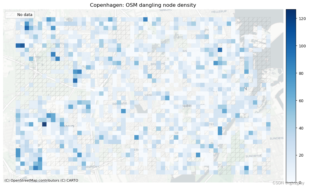
• 悬挂节点密度高于平均水平表明网格单元中存在相对较多的死角

全球网络密度

# Entire study area
edge_density, node_density, dangling_node_density = eval_func.compute_network_density((osm_edges_simplified, osm_nodes_simplified),grid.unary_union.area,return_dangling_nodes=True,
)density_results = {}
density_results["edge_density_m_sqkm"] = edge_density
density_results["node_density_count_sqkm"] = node_density
density_results["dangling_node_density_count_sqkm"] = dangling_node_densityosm_protected = osm_edges_simplified.loc[osm_edges_simplified.protected == "protected"]
osm_unprotected = osm_edges_simplified.loc[osm_edges_simplified.protected == "unprotected"
]
osm_mixed = osm_edges_simplified.loc[osm_edges_simplified.protected == "mixed"]osm_data = [osm_protected, osm_unprotected, osm_mixed]
labels = ["protected_density", "unprotected_density", "mixed_density"]for data, label in zip(osm_data, labels):if len(data) > 0:osm_edge_density_type, _ = eval_func.compute_network_density((data, osm_nodes_simplified),grid.unary_union.area,return_dangling_nodes=False,)density_results[label + "_m_sqkm"] = osm_edge_density_typeelse:density_results[label + "_m_sqkm"] = 0protected_edge_density = density_results["protected_density_m_sqkm"]
unprotected_edge_density = density_results["unprotected_density_m_sqkm"]
mixed_protection_edge_density = density_results["mixed_density_m_sqkm"]print(f"For the entire study area, there are:")
print(f"- {edge_density:.2f} meters of bicycle infrastructure per km2.")
print(f"- {node_density:.2f} nodes in the bicycle network per km2.")
print(f"- {dangling_node_density:.2f} dangling nodes in the bicycle network per km2."
)
print(f"- {protected_edge_density:.2f} meters of protected bicycle infrastructure per km2."
)
print(f"- {unprotected_edge_density:.2f} meters of unprotected bicycle infrastructure per km2."
)
print(f"- {mixed_protection_edge_density:.2f} meters of mixed protection bicycle infrastructure per km2."
)

For the entire study area, there are:
- 5824.58 meters of bicycle infrastructure per km2.
- 27.65 nodes in the bicycle network per km2.
- 10.08 dangling nodes in the bicycle network per km2.
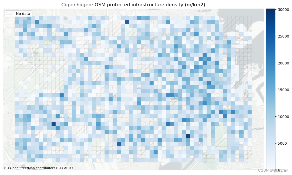
- 5342.41 meters of protected bicycle infrastructure per km2.
- 427.35 meters of unprotected bicycle infrastructure per km2.
- 54.82 meters of mixed protection bicycle infrastructure per km2.

# Save stats to csv
pd.DataFrame({"metric": ["meters of bicycle infrastructure per square km","nodes in the bicycle network per square km","dangling nodes in the bicycle network per square km","meters of protected bicycle infrastructure per square km","meters of unprotected bicycle infrastructure per square km","meters of mixed protection bicycle infrastructure per square km",],"value": [np.round(edge_density, 2),np.round(node_density, 2),np.round(dangling_node_density, 2),np.round(protected_edge_density, 2),np.round(unprotected_edge_density, 2),np.round(mixed_protection_edge_density, 2),],}
).to_csv(osm_results_data_fp + "stats_area.csv", index=False)

本地网络密度

# Per grid cell
results_dict = {}
data = (osm_edges_simp_joined, osm_nodes_simp_joined.set_index("osmid"))[eval_func.run_grid_analysis(grid_id,data,results_dict,eval_func.compute_network_density,grid["geometry"].loc[grid.grid_id == grid_id].area.values[0],return_dangling_nodes=True,)for grid_id in grid_ids
]results_df = pd.DataFrame.from_dict(results_dict, orient="index")
results_df.reset_index(inplace=True)
results_df.rename(columns={"index": "grid_id",0: "osm_edge_density",1: "osm_node_density",2: "osm_dangling_node_density",},inplace=True,
)grid = eval_func.merge_results(grid, results_df, "left")osm_protected = osm_edges_simp_joined.loc[osm_edges_simp_joined.protected == "protected"
]
osm_unprotected = osm_edges_simp_joined.loc[osm_edges_simp_joined.protected == "unprotected"
]
osm_mixed = osm_edges_simp_joined.loc[osm_edges_simp_joined.protected == "mixed"]osm_data = [osm_protected, osm_unprotected, osm_mixed]osm_labels = ["osm_protected_density", "osm_unprotected_density", "osm_mixed_density"]for data, label in zip(osm_data, osm_labels):if len(data) > 0:results_dict = {}data = (osm_edges_simp_joined.loc[data.index], osm_nodes_simp_joined)[eval_func.run_grid_analysis(grid_id,data,results_dict,eval_func.compute_network_density,grid["geometry"].loc[grid.grid_id == grid_id].area.values[0],)for grid_id in grid_ids]results_df = pd.DataFrame.from_dict(results_dict, orient="index")results_df.reset_index(inplace=True)results_df.rename(columns={"index": "grid_id", 0: label}, inplace=True)results_df.drop(1, axis=1, inplace=True)grid = eval_func.merge_results(grid, results_df, "left")

# Network density grid plotsset_renderer(renderer_map)
plot_cols = ["osm_edge_density", "osm_node_density", "osm_dangling_node_density"]
plot_titles = [area_name+": OSM edge density",area_name+": OSM node density",area_name+": OSM dangling node density",
]
filepaths = [osm_results_static_maps_fp + "density_edge_osm",osm_results_static_maps_fp + "density_node_osm",osm_results_static_maps_fp + "density_danglingnode_osm",
]
cmaps = [pdict["pos"], pdict["pos"], pdict["pos"]]
no_data_cols = ["count_osm_edges", "count_osm_nodes", "count_osm_nodes"]plot_func.plot_grid_results(grid=grid,plot_cols=plot_cols,plot_titles=plot_titles,filepaths=filepaths,cmaps=cmaps,alpha=pdict["alpha_grid"],cx_tile=cx_tile_2,no_data_cols=no_data_cols,
)

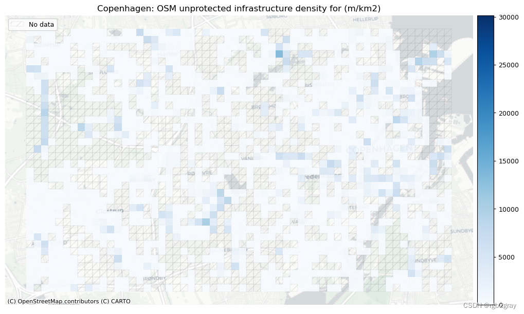
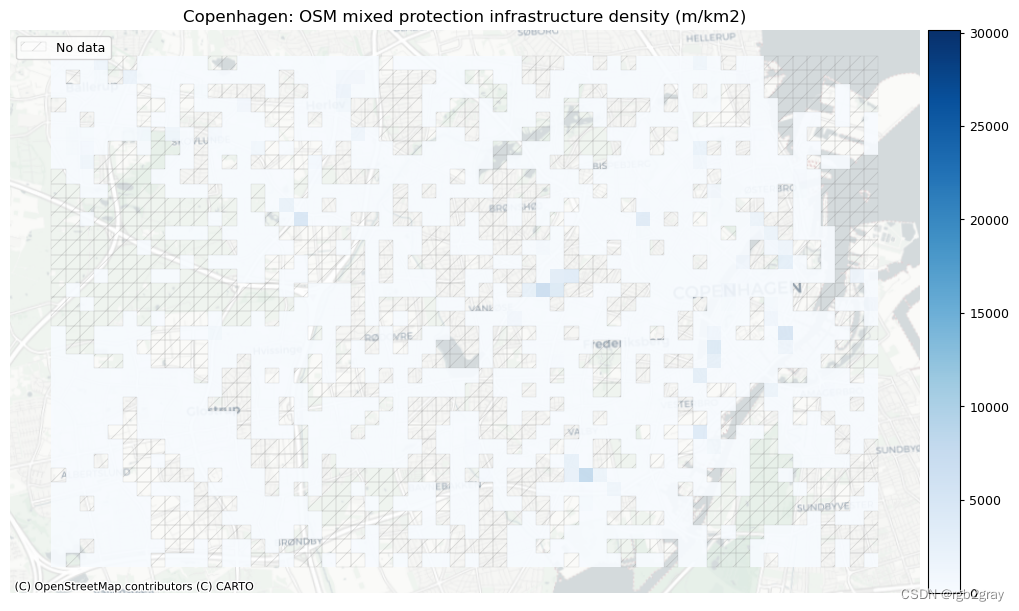
受保护和未受保护基础设施的密度

在 BikeDNA 中，“受保护的基础设施”是指通过高架路缘、护柱或其他物理屏障等与汽车交通分开的所有自行车基础设施，或者不毗邻街道的自行车道。

不受保护的基础设施是专门供骑自行车者使用的所有其他类型的车道，但仅通过汽车交通分隔，例如街道上的画线。

# Network density grid plotsset_renderer(renderer_map)
plot_cols = ["osm_protected_density", "osm_unprotected_density", "osm_mixed_density"]
plot_titles = [area_name+": OSM protected infrastructure density (m/km2)",area_name+": OSM unprotected infrastructure density for (m/km2)",area_name+": OSM mixed protection infrastructure density (m/km2)",
]
filepaths = [osm_results_static_maps_fp + "density_protected_osm",osm_results_static_maps_fp + "density_unprotected_osm",osm_results_static_maps_fp + "density_mixed_osm",
]cmaps = [pdict["pos"]] * len(plot_cols)
no_data_cols = ["osm_protected_density", "osm_unprotected_density", "osm_mixed_density"]
norm_min = [0] * len(plot_cols)
norm_max = [max(grid[plot_cols].fillna(value=0).max())] * len(plot_cols)plot_func.plot_grid_results(grid=grid,plot_cols=plot_cols,plot_titles=plot_titles,filepaths=filepaths,cmaps=cmaps,alpha=pdict["alpha_grid"],cx_tile=cx_tile_2,no_data_cols=no_data_cols,use_norm=True,norm_min=norm_min,norm_max=norm_max,
)

2.OSM标签分析

出于许多实际和研究目的，人们感兴趣的不仅仅是自行车基础设施的存在/不存在，还有更多的信息。 有关例如的信息 基础设施的宽度、速度限制、路灯等可能具有很高的相关性，例如在评估某个区域或单个网络段的自行车友好性时。 然而，这些描述自行车基础设施属性的标签在 OSM 中的分布非常不均匀，这对评估可骑自行车性和交通压力造成了障碍。 同样，对 OSM 特征标记方式缺乏限制有时会导致标记冲突，从而破坏循环条件的评估。

本节包括对缺失标签（带有缺乏信息的标签的边）、不兼容标签（带有两个或多个矛盾标签的标签的边）和标签模式（用于描述自行车基础设施的标签的空间变化）的分析。

对于标签的评估，应使用非简化边以避免在简化过程中聚合的标签出现问题。

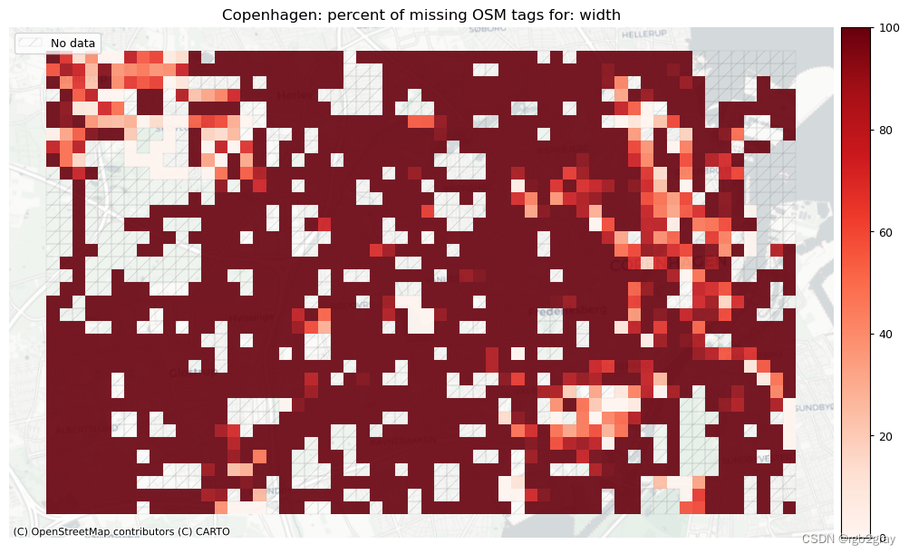
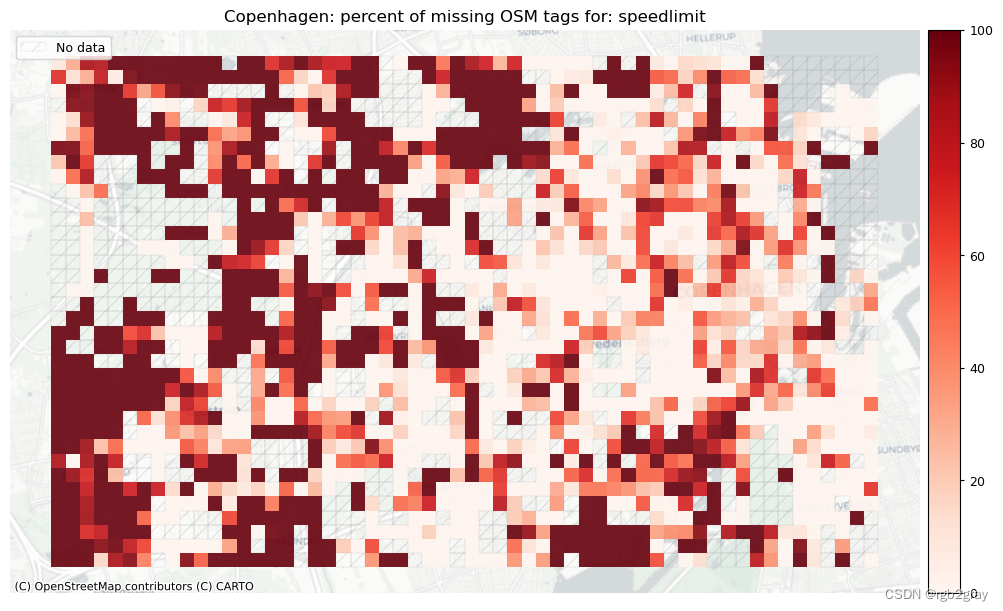
2.1 缺少标签

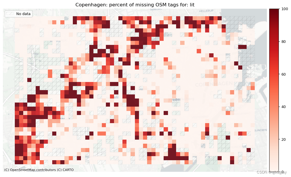
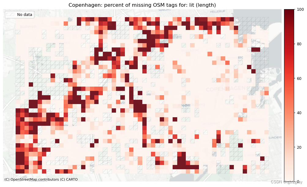
需要或希望从 OSM 标签获取的信息取决于用例 - 例如，研究自行车道上的光照条件的项目的标签“lit”。 下面的工作流程允许快速分析具有可用于感兴趣标签的值的网络边缘的百分比。

方法

我们分析“config.yml”的“existing_tag_analysis”部分中定义的所有感兴趣的标签。 对于每个标签，“analyze_existing_tags”用于计算具有相应标签值的边的总数和百分比。

解释

在研究区域级别，现有标签值的百分比越高，原则上表明数据集的质量越高。 然而，这与现有标签值是否真实的估计不同。 在网格单元级别上，现有标签值的百分比低于平均水平可能表明映射的区域更差。 然而，对于边数较少的网格单元来说，百分比的信息量较少：例如，如果单元格包含一个具有“lit”标签值的单边，则现有标签值的百分比为 100% - 但考虑到这一点 只有 1 个数据点，这比包含 200 条边的单元格的 80% 值提供的信息要少。

全局缺失标签

print(f"Analysing tags describing:")
for k in existing_tag_dict.keys():print(k, "-", end=" ")
print("\n")existing_tags_results = eval_func.analyze_existing_tags(osm_edges, existing_tag_dict)for key, value in existing_tags_results.items():print(f"{key}: {value['count']} out of {len(osm_edges)} edges ({value['count']/len(osm_edges)*100:.2f}%) have information.")print(f"{key}: {round(value['length']/1000)} out of {round(osm_edges.geometry.length.sum()/1000)} km ({100*value['length']/osm_edges.geometry.length.sum():.2f}%) have information.")print("\n")results_dict = {}
[eval_func.run_grid_analysis(grid_id,osm_edges_joined,results_dict,eval_func.analyze_existing_tags,existing_tag_dict,)for grid_id in grid_ids
]# compute the length of osm edges in each grid cell to use for pct missing tags based on length
grid_feature_len = eval_func.length_features_in_grid(osm_edges_joined, "osm_edges")
grid = eval_func.merge_results(grid, grid_feature_len, "left")restructured_results = {}for key, value in results_dict.items():unpacked_results = {}for tag, _ in existing_tag_dict.items():unpacked_results[tag + "_count"] = value[tag]["count"]unpacked_results[tag + "_length"] = value[tag]["length"]restructured_results[key] = unpacked_resultsresults_df = pd.DataFrame.from_dict(restructured_results, orient="index")
cols = results_df.columns
new_cols = ["existing_tags_" + c for c in cols]
results_df.columns = new_cols
results_df["existing_tags_sum"] = results_df[new_cols].sum(axis=1)
results_df.reset_index(inplace=True)
results_df.rename(columns={"index": "grid_id"}, inplace=True)grid = eval_func.merge_results(grid, results_df, "left")for c in new_cols:if "count" in c:grid[c + "_pct"] = round(grid[c] / grid.count_osm_edges * 100, 2)grid[c + "_pct_missing"] = 100 - grid[c + "_pct"]elif "length" in c:grid[c + "_pct"] = round(grid[c] / grid.length_osm_edges * 100, 2)grid[c + "_pct_missing"] = 100 - grid[c + "_pct"]existing_tags_pct = {}existing_tags_pct = {}for k, v in existing_tags_results.items():pct_dict = {}pct_dict["count_pct"] = (v["count"] / len(osm_edges)) * 100pct_dict["length_pct"] = (v["length"] / osm_edges.geometry.length.sum()) * 100existing_tags_pct[k] = pct_dictfor k, v in existing_tags_results.items():merged_results = v | existing_tags_pct[k]existing_tags_results[k] = merged_results

Analysing tags describing:
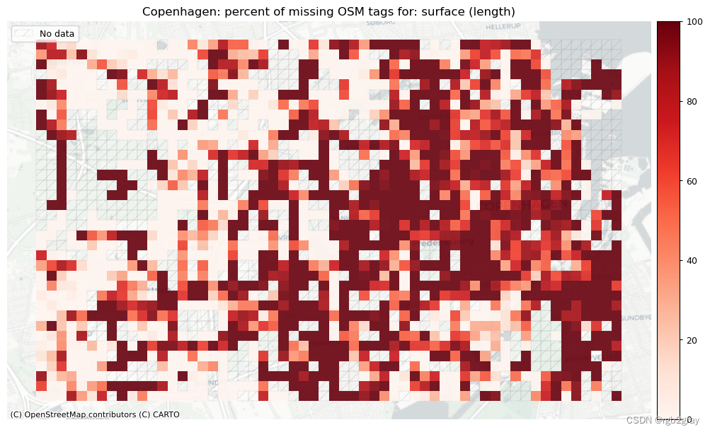
surface - width - speedlimit - lit - surface: 24821 out of 52168 edges (47.58%) have information.
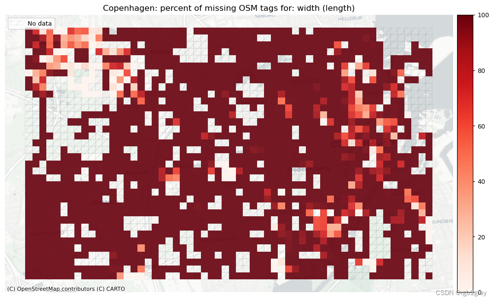
surface: 575 out of 1290 km (44.62%) have information.width: 6306 out of 52168 edges (12.09%) have information.
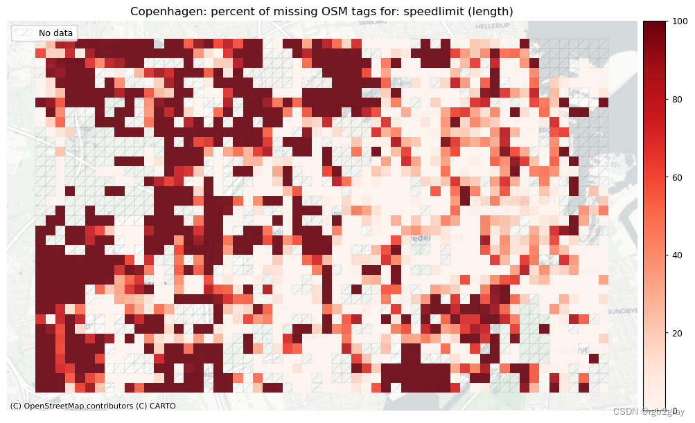
width: 111 out of 1290 km (8.57%) have information.speedlimit: 25498 out of 52168 edges (48.88%) have information.
speedlimit: 673 out of 1290 km (52.16%) have information.lit: 40759 out of 52168 edges (78.13%) have information.
lit: 1023 out of 1290 km (79.30%) have information.

# Save to csv# Initialize lists with values for entire data set
edgecount_list = [len(osm_edges)]
kmcount_list = [round(osm_edges.geometry.length.sum() / 1000)]
keys_list = ["TOTAL"]for key, value in existing_tags_results.items():keys_list.append(key)edgecount_list.append(value["count"])kmcount_list.append(round(value["length"] / 1000))pd.DataFrame({"tag": keys_list, "edge count": edgecount_list, "km (rounded)": kmcount_list}
).to_csv(osm_results_data_fp + "stats_tags.csv", index=False)

本地缺失标签

#  Plot pct missing for countset_renderer(renderer_map)
count_cols = [c for c in cols if 'count' in c]
filepaths = [osm_results_static_maps_fp + "tagsmissing_" + c + '_osm' for c in count_cols]
plot_cols = ["existing_tags_" + c + "_pct_missing" for c in count_cols]
count_cols = [c.removesuffix('_count') for c in count_cols]
plot_titles = [area_name+": percent of missing OSM tags for: " + c for c in count_cols]cmaps = [pdict["neg"]] * len(plot_cols)
no_data_cols = ["count_osm_edges"] * len(plot_cols)plot_func.plot_grid_results(grid=grid,plot_cols=plot_cols,plot_titles=plot_titles,filepaths=filepaths,cmaps=cmaps,alpha=pdict["alpha_grid"],cx_tile=cx_tile_2,no_data_cols=no_data_cols,
)

#  Plot pct missing based on the length of the edges with missing tagsset_renderer(renderer_map)
length_cols = [c for c in cols if 'length' in c]
plot_titles = [area_name+": percent of missing OSM tags for: " + c for c in length_cols]
filepaths = [osm_results_static_maps_fp + "tagsmissing_" + c + '_osm' for c in length_cols]
plot_cols = ["existing_tags_" + c + "_pct_missing" for c in length_cols]
plot_titles = [c.replace("_", " (") for c in plot_titles]
plot_titles = [c + ")" for c in plot_titles]cmaps = [pdict["neg"]] * len(plot_cols)
no_data_cols = ["count_osm_edges"] * len(plot_cols)plot_func.plot_grid_results(grid=grid,plot_cols=plot_cols,plot_titles=plot_titles,filepaths=filepaths,cmaps=cmaps,alpha=pdict["alpha_grid"],cx_tile=cx_tile_2,no_data_cols=no_data_cols,
)

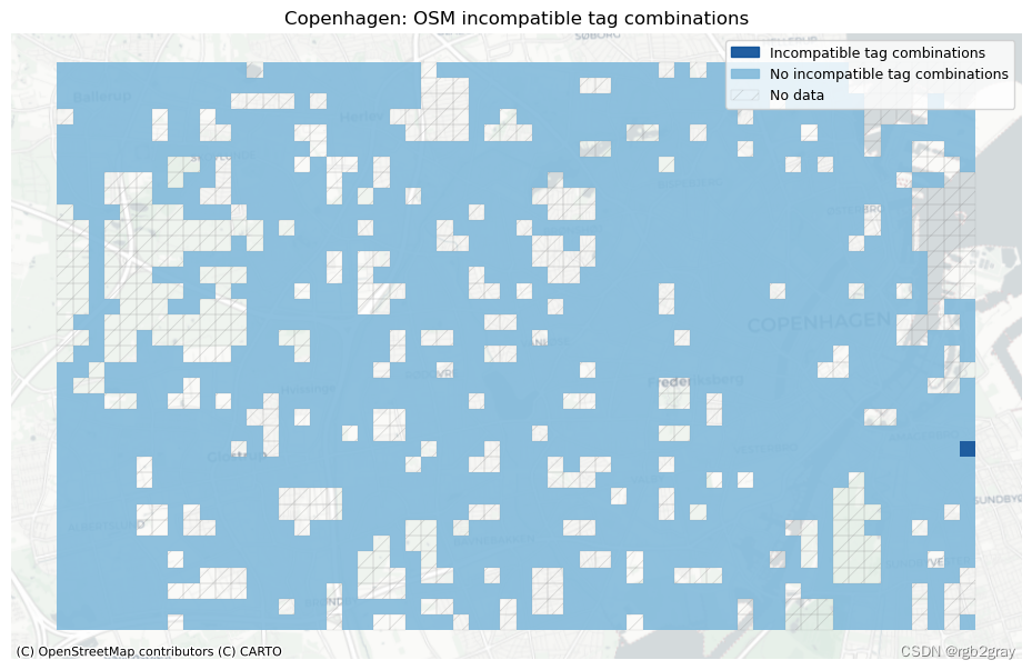
2.2 不兼容的标签

鉴于 OSM 数据中的标签有时缺乏一致性，并且标记过程没有限制（参见 Barron et al., 2014 ），数据集中可能存在不兼容的标签。 例如，一条边可能被标记为以下两个相互矛盾的键值对：“bicycle_infrastruct = yes”和“bicycle = no”。

方法

在“config.yml”文件中，定义了“incomplete_tags_analysis”中标签的不兼容键值对列表。 由于数据集可能包含的标签没有限制，因此根据定义，该列表并不详尽，并且可以由用户进行调整。 在下面的部分中，运行“check_inknown_tags”，它首先在研究区域级别上，然后在网格单元级别上识别给定区域的所有不兼容实例。

解释

不兼容的标签是数据集的一个不受欢迎的特征，并使相应的数据点无效； 没有直接的方法可以自动解决出现的问题，因此必须手动更正标签或从数据集中排除数据点。 网格单元中不兼容标签的数量高于平均水平表明存在局部映射问题。

全局不兼容标签（总数）

incompatible_tags_results = eval_func.check_incompatible_tags(osm_edges, incompatible_tags_dict, store_edge_ids=True
)print(f"In the entire data set, there are {sum(len(lst) for lst in incompatible_tags_results.values())} incompatible tag combinations (of those defined in the configuration file)."
)results_dict = {}
[eval_func.run_grid_analysis(grid_id,osm_edges_joined,results_dict,eval_func.check_incompatible_tags,incompatible_tags_dict,)for grid_id in grid_ids
]results_df = pd.DataFrame(index=results_dict.keys(), columns=results_dict[list(results_dict.keys())[0]].keys()
)for i in results_df.index:for j in results_df.columns:results_df.at[i, j] = results_dict[i][j]cols = results_df.columns
new_cols = ["incompatible_tags_" + c for c in cols]
results_df.columns = new_cols
results_df["incompatible_tags_sum"] = results_df[new_cols].sum(axis=1)
results_df.reset_index(inplace=True)
results_df.rename(columns={"index": "grid_id"}, inplace=True)
grid = eval_func.merge_results(grid, results_df, "left")

In the entire data set, there are 2 incompatible tag combinations (of those defined in the configuration file).

# Save to csv
df = pd.DataFrame(index=incompatible_tags_results.keys(), data=incompatible_tags_results.values()
)
edge_ids = []
for index, row in df.iterrows():edge_ids.append(row.to_list())df["edge_id"] = edge_ids
incomp_df = df[["edge_id"]]incomp_df.to_csv(osm_results_data_fp + "incompatible_tags.csv", index=True)

本地不兼容标签（每个网格单元）

# Overview plots (grid)if len(new_cols) > 0:set_renderer(renderer_map)fig, ax = plt.subplots(1, figsize=pdict["fsmap"])grid.loc[grid.incompatible_tags_sum == 0].plot(ax=ax, alpha=pdict["alpha_grid"], color=mpl.colors.rgb2hex(incompatible_false_patch.get_facecolor()))grid.loc[grid.incompatible_tags_sum > 0].plot(ax=ax, alpha=pdict["alpha_grid"], color=mpl.colors.rgb2hex(incompatible_true_patch.get_facecolor()))# add no data patchesgrid[grid["count_osm_edges"].isnull()].plot(ax=ax,facecolor=pdict["nodata_face"],edgecolor=pdict["nodata_edge"],linewidth= pdict["line_nodata"],hatch=pdict["nodata_hatch"],alpha=pdict["alpha_nodata"],)ax.legend(handles=[incompatible_true_patch, incompatible_false_patch, nodata_patch],loc="upper right",)ax.set_title(area_name+": OSM incompatible tag combinations")ax.set_axis_off()cx.add_basemap(ax=ax, crs=study_crs, source=cx_tile_2)plot_func.save_fig(fig, osm_results_static_maps_fp + "tagsincompatible_osm")else:print("There are no incompatible tag combinations to plot.")

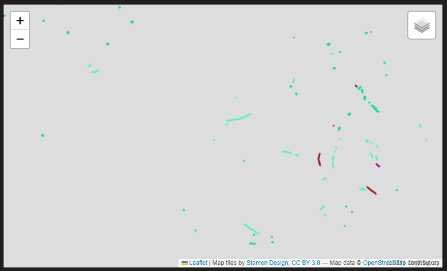
绘制不兼容的标签几何形状

incompatible_tags_edge_ids = eval_func.check_incompatible_tags(osm_edges, incompatible_tags_dict, store_edge_ids=True
)if len(incompatible_tags_edge_ids) > 0:incompatible_tags_fg = []# iterate through dict of queries,for i, key in enumerate(list(incompatible_tags_edge_ids.keys())):# create one feature group for each query# and append it to listincompatible_tags_fg.append(plot_func.make_edgefeaturegroup(gdf=osm_edges[osm_edges["edge_id"].isin(incompatible_tags_edge_ids[key])],mycolor=pdict["basecols"][i],myweight=pdict["line_emp"],nametag="Incompatible tags: " + key,show_edges=True,))### Make marker feature groupedge_ids = [itemfor sublist in list(incompatible_tags_edge_ids.values())for item in sublist]  # get ids of all edges that have incompatible tagsmfg = plot_func.make_markerfeaturegroup(osm_edges.loc[osm_edges["edge_id"].isin(edge_ids)], nametag="Incompatible tag marker", show_markers=True)incompatible_tags_fg.append(mfg)# create interactive mapm = plot_func.make_foliumplot(feature_groups=incompatible_tags_fg,layers_dict=folium_layers,center_gdf=osm_nodes,center_crs=osm_nodes.crs,)bounds = plot_func.compute_folium_bounds(osm_nodes_simplified)m.fit_bounds(bounds)m.save(osm_results_inter_maps_fp + "tagsincompatible_osm.html")display(m)

if len(incompatible_tags_edge_ids) > 0:print("Interactive map saved at " + osm_results_inter_maps_fp.lstrip("../") + "tagsincompatible_osm.html")
else:print("There are no incompatible tag combinations to plot.")

Interactive map saved at results/OSM/cph_geodk/maps_interactive/tagsincompatible_osm.html

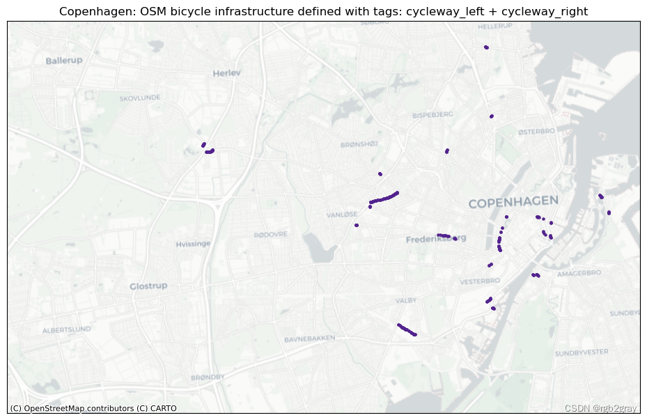
2.3 标记模式

由于可以通过多种不同的方式来指示自行车基础设施的存在，因此在 OSM 中识别自行车基础设施可能很棘手。 OSM Wiki 是一个很好的资源，提供了有关如何标记 OSM 功能的建议，但可能仍然存在一些不一致和局部变化。 对标记模式的分析可以直观地探索一些潜在的不一致之处。

无论自行车基础设施是如何定义的，检查哪些标签对自行车网络的哪些部分有贡献，都可以直观地检查标签方法中的模式。 它还允许估计查询的某些元素是否会导致包含太多或太少的特征。

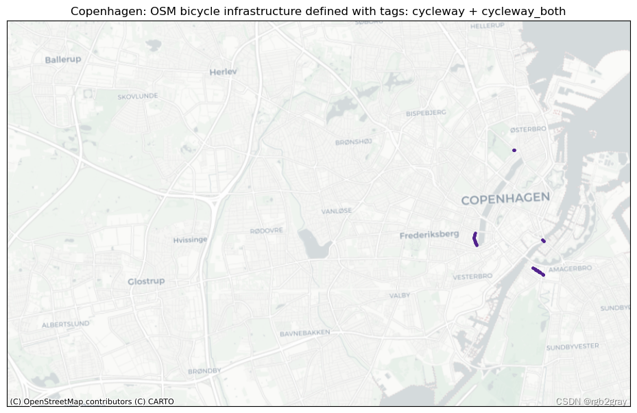
同样，使用多个不同标签来指示自行车基础设施的“双重标签”可能会导致数据错误分类。 因此，识别包含在多个定义自行车基础设施的查询中的特征可以表明标记质量存在问题。

方法

我们首先为“bicycle_infrastruction_queries”中列出的每个查询绘制 OSM 数据集的各个子集，如“config.yml”文件中所定义。 查询定义的子集是该查询为True的边的集合。 由于多个查询对于同一条边可能是“True”，因此子集可能会重叠。 在下面的第二步中，绘制两个或多个查询之间的所有重叠，即已分配多个可能竞争的标签的所有边。

解释

每种标记类型的图可以快速直观地概览该区域中存在的不同标记模式。 基于本地知识，用户可以估计标记类型的差异是由于基础设施中的实际物理差异还是OSM数据的人为造成的。 接下来，用户可以访问不同标签之间的重叠部分； 根据具体标签，这可能是也可能不是数据质量问题。 例如，在“cycleway:right”和“cycleway:left”的情况下，两个标签的数据都是有效的，但其他组合如“cycleway”=“track”和“cycleway:left” =lane’` 给出了关于自行车基础设施类型的模糊描述。

标记类型

osm_edges["tagging_type"] = ""for k, q in bicycle_infrastructure_queries.items():try:ox_filtered = osm_edges.query(q)except Exception:print("Exception occured when quering with:", q)osm_edges.loc[ox_filtered.index, "tagging_type"] = (osm_edges.loc[ox_filtered.index, "tagging_type"] + k)

# Interactive plot of tagging types# initialize list of folium feature groups (one per tagging type)
tagging_types_fg = []# iterate through dict of queries,
i = 0  # index for color change
for key in bicycle_infrastructure_queries.keys():# create one feature group for each query# and append it to listtagging_types_fg.append(plot_func.make_edgefeaturegroup(gdf=osm_edges[osm_edges["tagging_type"] == key],mycolor=pdict["basecols"][i],myweight=2,nametag="Tagging type " + key,show_edges=True,))i += 1  # update index# create interactive map
m = plot_func.make_foliumplot(feature_groups=tagging_types_fg,layers_dict=folium_layers,center_gdf=osm_nodes_simplified,center_crs=osm_nodes_simplified.crs,
)bounds = plot_func.compute_folium_bounds(osm_nodes_simplified)
m.fit_bounds(bounds)m.save(osm_results_inter_maps_fp + "taggingtypes_osm.html")for k, v in bicycle_infrastructure_queries.items():print("Tagging type " + k + ": " + v)display(m)

print("Interactive map saved at " + osm_results_inter_maps_fp.lstrip("../") + "taggingtypes_osm.html")

Interactive map saved at results/OSM/cph_geodk/maps_interactive/taggingtypes_osm.html

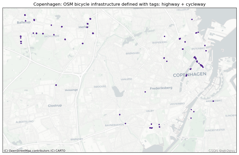
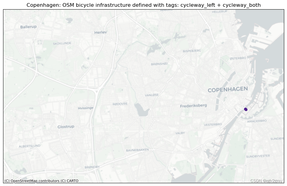
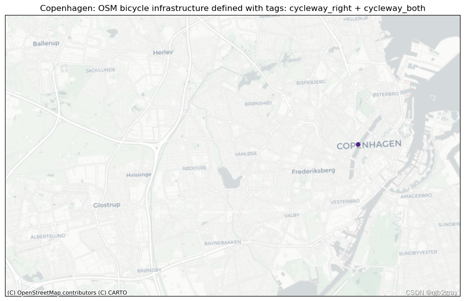
多重标记

# Plot all osm_edges which are returned for more than one tagging_typeset_renderer(renderer_map)
tagging_combinations = list(osm_edges.tagging_type.unique())
tagging_combinations = [x for x in tagging_combinations if len(x) > 1]if len(tagging_combinations) > 0:for i, t in enumerate(tagging_combinations):fig, ax = plt.subplots(1, figsize=pdict["fsmap"])ax.get_xaxis().set_visible(False)ax.get_yaxis().set_visible(False)if len(osm_edges.loc[osm_edges["tagging_type"] == t]) < 10:grid.plot(ax=ax, facecolor="none", edgecolor="none", alpha=0)osm_edges.loc[osm_edges["tagging_type"] == t]["geometry"].centroid.plot(ax=ax, color=pdict["osm_emp"], markersize=30)else:grid.plot(ax=ax, facecolor="none", edgecolor="none", alpha=0)osm_edges.loc[osm_edges["tagging_type"] == t]["geometry"].centroid.plot(ax=ax, color=pdict["osm_emp"], markersize=5)columns_in_query = ""for value in t:tag_name = bicycle_infrastructure_queries[value].split(" ")[0]columns_in_query = columns_in_query + tag_name + " + "columns_in_query = columns_in_query[:-3]title = area_name+": OSM bicycle infrastructure defined with tags: " + columns_in_queryax.set_title(title)cx.add_basemap(ax=ax, crs=study_crs, source=cx_tile_2)filepath_extension = columns_in_query.replace(" + ", "-")plot_func.save_fig(fig, osm_results_static_maps_fp + f"tagscompeting_{filepath_extension}_osm")plt.show()

if len(tagging_combinations) > 0:# set seed for colorsnp.random.seed(42)# generate enough random colors to plot all tagging combinationsrandcols = [colors.to_hex(rgbcol) for rgbcol in np.random.rand(len(tagging_combinations), 3)]# initialize list of feature groups (one for each tagging combination)tag_featuregroups = []for i, t in enumerate(tagging_combinations):columns_in_query = ""for value in t:tag_name = bicycle_infrastructure_queries[value].split(" ")[0]columns_in_query = columns_in_query + tag_name + " + "columns_in_query = columns_in_query[:-3]tag_featuregroup = plot_func.make_edgefeaturegroup(gdf=osm_edges.loc[osm_edges["tagging_type"] == t],mycolor=randcols[i],myweight=pdict["line_emp"],nametag=columns_in_query,show_edges=True,)tag_featuregroups.append(tag_featuregroup)m = plot_func.make_foliumplot(feature_groups=tag_featuregroups,layers_dict=folium_layers,center_gdf=osm_nodes_simplified,center_crs=osm_nodes_simplified.crs,)bounds = plot_func.compute_folium_bounds(osm_nodes_simplified)m.fit_bounds(bounds)m.save(osm_results_inter_maps_fp + "taggingcombinations_osm.html") display(m)

if len(tagging_combinations) > 0:print("Interactive map saved at " + osm_results_inter_maps_fp.lstrip("../") + "taggingcombinations_osm.html")
else:print("There are no tagging combinations to plot.")

Interactive map saved at results/OSM/cph_geodk/maps_interactive/taggingcombinations_osm.html

3.网络拓扑结构

4.网络组件

5.概括

6.保存结果

其余部分见BikeDNA（三） OSM数据的内在分析2

这篇关于BikeDNA（二） OSM数据的内在分析1的文章就介绍到这儿，希望我们推荐的文章对编程师们有所帮助！

---