本文主要是介绍Kaggle-水果图像分类银奖项目 pytorch Densenet GoogleNet ResNet101 VGG19,希望对大家解决编程问题提供一定的参考价值,需要的开发者们随着小编来一起学习吧!
一些原理文章
卷积神经网络基础(卷积,池化,激活,全连接) - 知乎
PyTorch 入门与实践(六)卷积神经网络进阶(DenseNet)_pytorch conv1x1_Skr.B的博客-CSDN博客
GoogLeNet网络结构的实现和详解_Dragon_0010的博客-CSDN博客
一文读懂LeNet、AlexNet、VGG、GoogleNet、ResNet到底是什么? - 知乎
使用PyTorch搭建ResNet101、ResNet152网络_torch resnet101-CSDN博客
深度学习之VGG19模型简介-CSDN博客
Georgiisirotenko的银奖原始代码
PyTorch|Fruits|TransferLearing+Ensemble|Test99.18% | Kaggle
调用模型
torchvision.models.densenet121、torchvision.models.googlenet、torchvision.models.resnet101、torchvision.models.vgg19_bn
结果图
预测概率
部分打分
本地可运行代码
#https://www.kaggle.com/code/georgiisirotenko/pytorch-fruits-transferlearing-ensemble-test99-18
#!/usr/bin/env python
# coding: utf-8# # **0. Importing Libraries**# In[2]:
%pip install mlxtend
%pip install opencv-python -i https://pypi.tuna.tsinghua.edu.cn/simple
#可能需要重启kernel
# In[3]:
import numpy as np
import pandas as pd
import os
import random
from operator import itemgetter
import cv2
import copy
import timeimport matplotlib.pyplot as plt
import matplotlib.image as mpimg
from matplotlib.image import imread
import seaborn as snsimport torch
import torchvision
from torchvision.datasets import ImageFolderfrom torchvision.utils import make_grid
import torchvision.transforms as transform
from torch.utils.data import Dataset, DataLoader, ConcatDataset
from sklearn.model_selection import train_test_split
import torch.nn as nn
import torchvision.models as models
from torchvision.utils import make_grid
import torch.nn.functional as Ffrom mlxtend.plotting import plot_confusion_matrix
from sklearn.metrics import confusion_matrix, classification_reportimport warnings
warnings.filterwarnings('ignore')device = torch.device('cuda:0' if torch.cuda.is_available() else 'cpu')# # **1. Data loading and preparation¶**
# **Paths**# In[4]:example_train_path = './datadev/train/'
path = './datadev/'# **Show example from data and size**# In[5]:img = mpimg.imread(example_train_path + "0/60695900831062008.jpg")
print("Shape:", img.shape)
plt.imshow(img);# **Sometimes the data is normalized in advance, but as you can see in the graph, this is not the case, so the data will have to be normalized**# In[6]:def plotHist(img):plt.figure(figsize=(10,5))plt.subplot(1,2,1)plt.imshow(img, cmap='gray')plt.axis('off')histo = plt.subplot(1,2,2)histo.set_ylabel('Count')histo.set_xlabel('Pixel Intensity')plt.hist(img.flatten(), bins=10, lw=0, color='r', alpha=0.5)plotHist(img)# **Normalize and load the data**# In[7]:transformer = transform.Compose([transform.ToTensor(),transform.Normalize([0.6840562224388123, 0.5786514282226562, 0.5037682056427002],[0.3034113645553589, 0.35993242263793945, 0.39139702916145325])])# In[8]:bs = 50training = ImageFolder(path+'/train', transform=transformer)trainset, valset = train_test_split(training, test_size=0.05, shuffle=True, random_state=9)loaders = {'train':DataLoader(trainset, batch_size=bs, num_workers=4, pin_memory=False), #, num_workers=4, pin_memory=False'val': DataLoader(valset, batch_size=bs, num_workers=4, pin_memory=False)}dataset_sizes = {'train':len(trainset), 'val':len(valset)}# **Let's check the average and standard deviation of the images for each channel. As we can observe, the standard deviation is near one, and the mean is near zero, which is what we need**# In[9]:channels = 3for channel in range(channels):for x in ['train', 'val']:#number of pixels in the dataset = number of all pixels in one object * number of all objects in the datasetnum_pxl = dataset_sizes[x]*100*100#we go through the butches and sum up the pixels of the objects, #which then divide the sum by the number of all pixels to calculate the averagetotal_sum = 0for batch in loaders[x]:layer = list(map(itemgetter(channel), batch[0]))layer = torch.stack(layer, dim=0)total_sum += layer.sum()mean = total_sum / num_pxl#we calculate the standard deviation using the formula that I indicated abovesum_sqrt = 0for batch in loaders[x]: layer = list(map(itemgetter(channel), batch[0]))sum_sqrt += ((torch.stack(layer, dim=0) - mean).pow(2)).sum()std = torch.sqrt(sum_sqrt / num_pxl)print(f'|channel:{channel+1}| {x} - mean: {mean}, std: {std}')# In[10]:x, y = next(iter(loaders['train']))
x.mean(), x.std()# In[11]:x, y = next(iter(loaders['train']))
img_norm = x[0].permute(1,2,0).numpy()
plotHist(img_norm)# **So we can see the number of classes, there are really a lot of them**# In[12]:len(training.classes)# **Since information is always better perceived visually, I will make a graph with the distribution of classes**# In[13]:dic = {}for classes in training.classes:for filename in os.listdir(path+'/train/'+classes):dic[classes] = [len([os.path.join(path+'/train/'+classes, filename) for filename in os.listdir(path+'/train/'+classes)])]train_samplesize = pd.DataFrame.from_dict(dic)# In[14]:train_samplesize# In[15]:figure_size = plt.rcParams["figure.figsize"]
figure_size[0] = 40
figure_size[1] = 20
plt.rcParams["figure.figsize"] = figure_sizesns.barplot(data=train_samplesize)index = np.arange(len(training.classes))plt.xlabel('Fruits', fontsize=25)
plt.ylabel('Count of Fruits', fontsize=25)
plt.xticks(index, training.classes, fontsize=15, rotation=90)
plt.title('Training Set Distrubution', fontsize=35)
plt.show()# **Let's look at the data itself, which we will need to work with**# In[16]:# Function for plotting samples
def plot_samples(samples): fig, ax = plt.subplots(nrows=5, ncols=5, figsize=(15,12))i = 0for row in range(5):for col in range(5):img = mpimg.imread(samples[i][0][0])ax[row][col].imshow(img)ax[row][col].axis('off')ax[row][col].set_title(samples[i][1], fontsize=15)i+=1rand_samples = []
for _ in range(25): classes = random.choice(training.classes)rand_samples.append([random.sample([os.path.join(path+'/train/'+classes, filename) for filename in os.listdir(path+'/train/'+classes)], 1), classes])
rand_samples[0]
plot_samples(rand_samples)
plt.suptitle('Training Set Samples', fontsize=30)
plt.show()# # **3. Training**
# **I will use an ensemble of pre-trained models, the idea is this: I first train only the classifier on 10 epochs, then unfreeze the network and train all together for another 10 epochs**# **Let's write the accuracy function so that we don't have to write it several times**# In[17]:def accuracy(outputs, labels):_, preds = torch.max(outputs, dim=1) return torch.tensor(torch.sum(preds == labels).item() / len(preds)), preds# **Learning history for further visualization**# In[18]:#save the losses for further visualization
losses = {'train':[], 'val':[]}
accuracies = {'train':[], 'val':[]}# Train function structure:
#
# 1. **Classifier Training**
# 2. **Network-wide Training**# In[19]:def train(seed, epochs, model):print('Creating a model {}...'.format(seed))model.to(device) criterion = nn.CrossEntropyLoss()if seed==2 or seed==3:optimizer = torch.optim.Adam(model.fc.parameters(), lr=0.001, betas=(0.9, 0.999), eps=1e-08, weight_decay=0)else:optimizer = torch.optim.Adam(model.classifier.parameters(), lr=0.001, betas=(0.9, 0.999), eps=1e-08, weight_decay=0)scheduler = torch.optim.lr_scheduler.ReduceLROnPlateau(optimizer, mode='max', factor=0.1, patience=3, verbose=True)scheduler = torch.optim.lr_scheduler.StepLR(optimizer, 4, gamma=0.1)since = time.time()best_model = copy.deepcopy(model.state_dict())best_acc = 0.0for epoch in range(epochs):for phase in ['train', 'val']:if phase == 'train':model.train()else:model.eval()running_loss = 0.0running_corrects = 0.0for inputs, labels in loaders[phase]:inputs, labels = inputs.to(device), labels.to(device)optimizer.zero_grad()with torch.set_grad_enabled(phase=='train'):outp = model(inputs)_, pred = torch.max(outp, 1)loss = criterion(outp, labels)if phase == 'train':loss.backward()optimizer.step()running_loss += loss.item()*inputs.size(0)running_corrects += torch.sum(pred == labels.data)if phase == 'train':acc = 100. * running_corrects.double() / dataset_sizes[phase]scheduler.step(acc)epoch_loss = running_loss / dataset_sizes[phase]epoch_acc = running_corrects.double()/dataset_sizes[phase]losses[phase].append(epoch_loss)accuracies[phase].append(epoch_acc)if phase == 'train':print('Epoch: {}/{}'.format(epoch+1, epochs))print('{} - loss:{}, accuracy{}'.format(phase, epoch_loss, epoch_acc))if phase == 'val':print('Time: {}m {}s'.format((time.time()- since)//60, (time.time()- since)%60))print('=='*31)if phase == 'val' and epoch_acc > best_acc:best_acc = epoch_accbest_model = copy.deepcopy(model.state_dict())#scheduler.step() time_elapsed = time.time() - sinceprint('CLASSIFIER TRAINING TIME {}m {}s'.format(time_elapsed//60, time_elapsed%60))print('=='*31)model.load_state_dict(best_model)for param in model.parameters():param.requires_grad=Trueoptimizer = torch.optim.Adam(model.parameters(), lr=0.0001, betas=(0.9, 0.999), eps=1e-08, weight_decay=0) scheduler = torch.optim.lr_scheduler.ReduceLROnPlateau(optimizer, factor=0.1, patience=2, verbose=True)#scheduler = torch.optim.lr_scheduler.StepLR(optimizer, 4, gamma=0.1)for epoch in range(epochs):for phase in ['train', 'val']:if phase == 'train':model.train()else:model.eval()running_loss = 0.0running_corrects = 0.0for inputs, labels in loaders[phase]:inputs, labels = inputs.to(device), labels.to(device)optimizer.zero_grad()with torch.set_grad_enabled(phase=='train'):outp = model(inputs)_, pred = torch.max(outp, 1)loss = criterion(outp, labels)if phase == 'train':loss.backward()optimizer.step()running_loss += loss.item()*inputs.size(0)running_corrects += torch.sum(pred == labels.data)if phase == 'train':acc = 100. * running_corrects.double() / dataset_sizes[phase]scheduler.step(acc)epoch_loss = running_loss / dataset_sizes[phase]epoch_acc = running_corrects.double()/dataset_sizes[phase]losses[phase].append(epoch_loss)accuracies[phase].append(epoch_acc)if phase == 'train':print('Epoch: {}/{}'.format(epoch+1, epochs))print('{} - loss:{}, accuracy{}'.format(phase, epoch_loss, epoch_acc))if phase == 'val':print('Time: {}m {}s'.format((time.time()- since)//60, (time.time()- since)%60))print('=='*31) if phase == 'val' and epoch_acc > best_acc:best_acc = epoch_accbest_model = copy.deepcopy(model.state_dict())#scheduler.step() time_elapsed = time.time() - sinceprint('ALL NET TRAINING TIME {}m {}s'.format(time_elapsed//60, time_elapsed%60))print('=='*31)model.load_state_dict(best_model)return model# **Uploading models**# In[20]:
densenet121_0 = torchvision.models.densenet121(pretrained=True)
for param in densenet121_0.parameters():param.requires_grad=False
densenet121_0.classifier = nn.Linear(in_features=densenet121_0.classifier.in_features, out_features=len(training.classes), bias=True)# In[21]:
densenet121_1 = torchvision.models.densenet121(pretrained=True)
for param in densenet121_1.parameters():param.requires_grad=False
densenet121_1.classifier = nn.Linear(in_features=densenet121_1.classifier.in_features, out_features=len(training.classes), bias=True)# In[22]:
googlenet = torchvision.models.googlenet(pretrained=True)
for param in googlenet.parameters():param.grad_requires = False
googlenet.fc = nn.Linear(in_features=googlenet.fc.in_features, out_features=len(training.classes), bias=True)# In[23]:
resnet101 = torchvision.models.resnet101(pretrained=True)
for param in resnet101.parameters():param.grad_requires = False
resnet101.fc = nn.Linear(in_features=resnet101.fc.in_features, out_features=len(training.classes), bias=True)# In[24]:
vgg19_bn = torchvision.models.vgg19_bn(pretrained=True)
for param in vgg19_bn.parameters():param.grad_requires = False
vgg19_bn.classifier[6] = nn.Linear(4096, len(training.classes), bias=True)# In[25]:
# torch.save(densenet121_0.state_dict(), 'densenet121_0.pth')
# torch.save(densenet121_1.state_dict(), 'densenet121_1.pth')
# torch.save(googlenet.state_dict(), 'googlenet.pth')
# torch.save(resnet101.state_dict(), 'resnet101.pth')
# torch.save(vgg19_bn.state_dict(), 'vgg19_bn.pth')# In[26]:
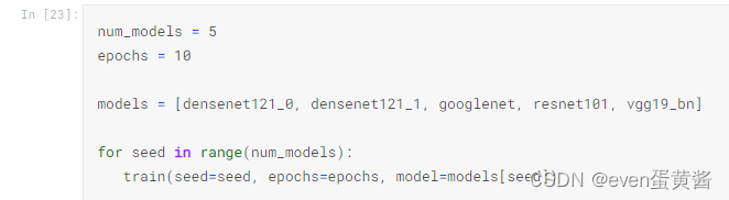
# **Launching training**
num_models = 5
epochs = 10
models = [densenet121_0, densenet121_1, googlenet, resnet101, vgg19_bn]
for seed in range(num_models):train(seed=seed, epochs=epochs, model=models[seed])
# In[38]:
# # **4. Test**
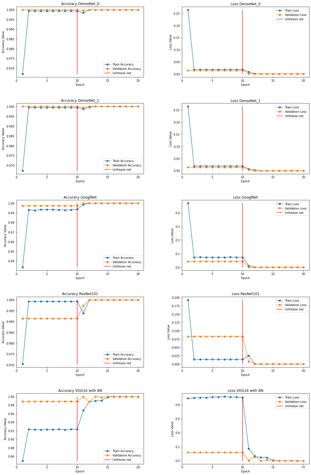
# **Visualization of training. As we can see, after defrosting, the indicators have improved**
fig, ax = plt.subplots(5, 2, figsize=(15, 15))
modelname = ['DenseNet_0', 'DenseNet_1', 'GooglNet', 'ResNet101', 'VGG19 with BN']
epochs=10
i=0
for row in range(5):trainaccarr=[]valaccarr=[]trainlosarr=[]vallosarr=[]for k in range(20):trainaccarr.append(accuracies['train'][i+k].item())valaccarr.append(accuracies['val'][i+k].item())trainlosarr.append(losses['train'][i+k])vallosarr.append(losses['val'][i+k])epoch_list = list(range(1,epochs*2+1))ax[row][0].plot(epoch_list, trainaccarr, '-o', label='Train Accuracy')ax[row][0].plot(epoch_list, valaccarr, '-o', label='Validation Accuracy')ax[row][0].plot([epochs for x in range(20)], np.linspace(min(trainaccarr), max(trainaccarr), 20), color='r', label='Unfreeze net')ax[row][0].set_xticks(np.arange(0, epochs*2+1, 5))ax[row][0].set_ylabel('Accuracy Value')ax[row][0].set_xlabel('Epoch')ax[row][0].set_title('Accuracy {}'.format(modelname[row]))ax[row][0].legend(loc="best")ax[row][1].plot(epoch_list, trainlosarr, '-o', label='Train Loss')ax[row][1].plot(epoch_list, vallosarr, '-o',label='Validation Loss')ax[row][1].plot([epochs for x in range(20)], np.linspace(min(trainlosarr), max(trainlosarr), 20), color='r', label='Unfreeze net')ax[row][1].set_xticks(np.arange(0, epochs*2+1, 5))ax[row][1].set_ylabel('Loss Value')ax[row][1].set_xlabel('Epoch')ax[row][1].set_title('Loss {}'.format(modelname[row]))ax[row][1].legend(loc="best")fig.tight_layout()fig.subplots_adjust(top=1.5, wspace=0.3)i+=20# **Let's write a model class that contains 5 already trained models**# In[39]:class Ensemble(nn.Module):def __init__(self, device):super(Ensemble,self).__init__()# you should use nn.ModuleList. Optimizer doesn't detect python list as parametersself.models = nn.ModuleList(models)def forward(self, x):# it is super simple. just forward num_ models and concat it.output = torch.zeros([x.size(0), len(training.classes)]).to(device)for model in self.models:output += model(x)return output# In[40]:model = Ensemble(device)# **Let's write some functions that will help us make predictions and load the test data**# In[41]:def validation_step(batch):images,labels = batchimages,labels = images.to(device),labels.to(device)out = model(images) loss = F.cross_entropy(out, labels) acc,preds = accuracy(out, labels) return {'val_loss': loss.detach(), 'val_acc':acc.detach(), 'preds':preds.detach(), 'labels':labels.detach()}# In[42]:def test_prediction(outputs):batch_losses = [x['val_loss'] for x in outputs]epoch_loss = torch.stack(batch_losses).mean() batch_accs = [x['val_acc'] for x in outputs]epoch_acc = torch.stack(batch_accs).mean() # combine predictionsbatch_preds = [pred for x in outputs for pred in x['preds'].tolist()] # combine labelsbatch_labels = [lab for x in outputs for lab in x['labels'].tolist()] return {'test_loss': epoch_loss.item(), 'test_acc': epoch_acc.item(),'test_preds': batch_preds, 'test_labels': batch_labels}# In[43]:@torch.no_grad()
def test_predict(model, test_loader):model.eval()# perform testing for each batchoutputs = [validation_step(batch) for batch in test_loader] results = test_prediction(outputs) print('test_loss: {:.4f}, test_acc: {:.4f}'.format(results['test_loss'], results['test_acc']))return results['test_preds'], results['test_labels']# In[44]:testset = ImageFolder(path+'/test', transform=transformer)# In[45]:test_dl = DataLoader(testset, batch_size=256)
model.to(device)
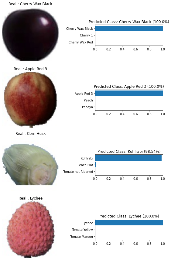
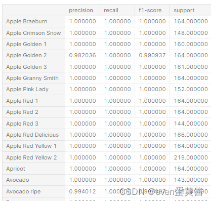
preds,labels = test_predict(model, test_dl)# # **4. Metrics**# **To visualize the data qualitatively, we need to normalize it back, that is, to return the pixel brightness distribution to its original state. This is what the function below does**# In[46]:def norm_out(img):img = img.permute(1,2,0)mean = torch.FloatTensor([0.6840562224388123, 0.5786514282226562, 0.5037682056427002])std = torch.FloatTensor([0.3034113645553589, 0.35993242263793945, 0.39139702916145325])img = img*std + meanreturn np.clip(img,0,1)# **Let's see how confident the network is in its predictions, as you can see, the network has trained well and gives confident predictions**# In[47]:fig, ax = plt.subplots(figsize=(8,12), ncols=2, nrows=4)for row in range(4):i = np.random.randint(0, high=len(testset))img,label = testset[i]m = nn.Softmax(dim=1)percent = m(model(img.to(device).unsqueeze(0)))predmax3percent = torch.sort(percent[0])[0][-3:]predmax3inds = torch.sort(percent[0])[1][-3:]classes = np.array([training.classes[predmax3inds[-3]], training.classes[predmax3inds[-2]],training.classes[predmax3inds[-1]]])class_name = training.classesax[row][0].imshow(norm_out(img))ax[row][0].set_title('Real : {}'.format(class_name[label]))ax[row][0].axis('off')ax[row][1].barh(classes, predmax3percent.detach().cpu().numpy())ax[row][1].set_aspect(0.1)ax[row][1].set_yticks(classes)ax[row][1].set_title('Predicted Class: {} ({}%)'.format(training.classes[predmax3inds[-1]], round((predmax3percent[-1]*100).item(), 2)))ax[row][1].set_xlim(0, 1.)plt.tight_layout()# **Here you can see the main metrics for each individual class**# In[48]:report = classification_report(labels, preds,output_dict=True,target_names=training.classes)
report_df = pd.DataFrame(report).transpose()# In[49]:pd.set_option("display.max_rows", None)
report_df.head(134)# ***I am always happy to receive any feedback. What do you think can be changed and what can be removed?***
这篇关于Kaggle-水果图像分类银奖项目 pytorch Densenet GoogleNet ResNet101 VGG19的文章就介绍到这儿,希望我们推荐的文章对编程师们有所帮助!


