本文主要是介绍金融量化 - 技术分析策略和交易系统_SMA+CCI交易系统,希望对大家解决编程问题提供一定的参考价值,需要的开发者们随着小编来一起学习吧!
双技术指标:SMA+CCI交易系统
以SMA作为开平仓信号,同时增加CCI作为过滤器;
当股价上穿SMA,同时CCI要小于-100,说明是在超卖的情况下,上穿SMA,做多;交易信号更可信;
当股价下穿SMA,同时CCI要大于+100,说明是在超买的情况下,下穿SMA,做空;交易信号更可信;
import numpy as np
import pandas as pd
import talib as ta
import tushare as ts
import matplotlib as mpl
import matplotlib.pyplot as plt
import seaborn as sns
%matplotlib inline
# 确保‘-’号显示正常
mpl.rcParams['axes.unicode_minus']=False
# 确保中文显示正常
mpl.rcParams['font.sans-serif'] = ['SimHei']
1. 数据准备
# 获取数据
stock_index = ts.get_k_data('hs300', '2016-01-01', '2017-06-30')
stock_index.set_index('date', inplace=True)
stock_index.sort_index(inplace = True)
stock_index.head()
| open | close | high | low | volume | code | |
|---|---|---|---|---|---|---|
| date | ||||||
| 2016-01-04 | 3725.86 | 3470.41 | 3726.25 | 3469.01 | 115370674.0 | hs300 |
| 2016-01-05 | 3382.18 | 3478.78 | 3518.22 | 3377.28 | 162116984.0 | hs300 |
| 2016-01-06 | 3482.41 | 3539.81 | 3543.74 | 3468.47 | 145966144.0 | hs300 |
| 2016-01-07 | 3481.15 | 3294.38 | 3481.15 | 3284.74 | 44102641.0 | hs300 |
| 2016-01-08 | 3371.87 | 3361.56 | 3418.85 | 3237.93 | 185959451.0 | hs300 |
# 计算指标sma,cci
stock_index['sma'] = ta.SMA(np.asarray(stock_index['close']), 5)
stock_index['cci'] = ta.CCI(np.asarray(stock_index['high']), np.asarray(stock_index['low']), np.asarray(stock_index['close']), timeperiod=20)
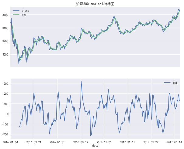
plt.subplot(2,1,1)
plt.title('沪深300 sma cci指标图')
plt.gca().axes.get_xaxis().set_visible(False)
stock_index['close'].plot(figsize = (10,8))
stock_index['sma'].plot(figsize=(10,8))
plt.legend()
plt.subplot(2,1,2)
stock_index['cci'].plot(figsize = (10,8))
plt.legend()
plt.show()
2. 交易信号、持仓信号和策略逻辑
2.1 交易信号
# 产生开仓信号时应使用昨日及前日数据,以避免未来数据
stock_index['yes_close'] = stock_index['close'].shift(1)
stock_index['yes_sma'] = stock_index['sma'].shift(1)
stock_index['yes_cci'] = stock_index['cci'].shift(1)   #CCI是作为策略的一个过滤器;
stock_index['daybeforeyes_close'] = stock_index['close'].shift(2)
stock_index['daybeforeyes_sma'] = stock_index['sma'].shift(2)
stock_index.head()
# 产生交易信号
# sma开多信号:昨天股价上穿SMA;
stock_index['sma_signal'] = np.where(np.logical_and(stock_index['daybeforeyes_close']<stock_index['daybeforeyes_sma'],stock_index['yes_close']>stock_index['yes_sma']), 1, 0)
# sma开空信号:昨天股价下穿SMA
stock_index['sma_signal'] = np.where(np.logical_and(stock_index['daybeforeyes_close']>stock_index['daybeforeyes_sma'],stock_index['yes_close']<stock_index['yes_sma']),-1,stock_index['sma_signal'])
# 产生cci做多过滤信号
stock_index['cci_filter'] = np.where(stock_index['yes_cci'] < -100, 1, 0)
# 产生cci做空过滤信号
stock_index['cci_filter'] = np.where(stock_index['yes_cci'] > 100,-1, stock_index['cci_filter'])
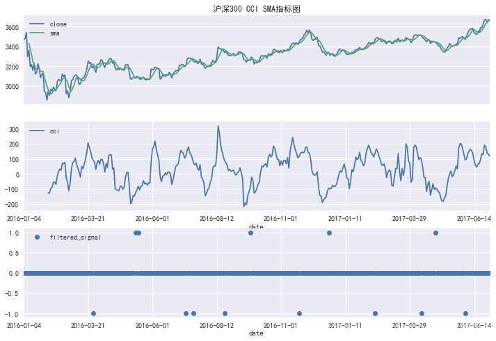
# 过滤后的开多信号
stock_index['filtered_signal'] = np.where(stock_index['sma_signal']+stock_index['cci_filter']==2, 1, 0)
# 过滤后的开空信号
stock_index['filtered_signal'] = np.where(stock_index['sma_signal']+stock_index['cci_filter']==-2, -1,stock_index['filtered_signal'])
# 生成交易信号stock_index.tail()
| open | close | high | low | volume | code | sma | cci | yes_close | yes_sma | yes_cci | daybeforeyes_close | daybeforeyes_sma | sma_signal | cci_filter | filtered_signal | |
|---|---|---|---|---|---|---|---|---|---|---|---|---|---|---|---|---|
| date | ||||||||||||||||
| 2017-06-26 | 3627.02 | 3668.09 | 3671.94 | 3627.02 | 134637995.0 | hs300 | 3603.152 | 190.662244 | 3622.88 | 3580.268 | 127.766972 | 3590.34 | 3559.444 | 0 | -1 | 0 |
| 2017-06-27 | 3665.58 | 3674.72 | 3676.53 | 3648.76 | 97558702.0 | hs300 | 3628.798 | 180.056339 | 3668.09 | 3603.152 | 190.662244 | 3622.88 | 3580.268 | 0 | -1 | 0 |
| 2017-06-28 | 3664.16 | 3646.17 | 3672.19 | 3644.03 | 97920858.0 | hs300 | 3640.440 | 138.038475 | 3674.72 | 3628.798 | 180.056339 | 3668.09 | 3603.152 | 0 | -1 | 0 |
| 2017-06-29 | 3649.25 | 3668.83 | 3669.13 | 3644.73 | 85589498.0 | hs300 | 3656.138 | 130.685000 | 3646.17 | 3640.440 | 138.038475 | 3674.72 | 3628.798 | 0 | -1 | 0 |
| 2017-06-30 | 3654.73 | 3666.80 | 3669.76 | 3646.23 | 81510028.0 | hs300 | 3664.922 | 118.314672 | 3668.83 | 3656.138 | 130.685000 | 3646.17 | 3640.440 | 0 | -1 | 0 |
# 绘制cci,sma指标图
plt.subplot(3,1,1)
plt.title('沪深300 CCI SMA指标图')
plt.gca().axes.get_xaxis().set_visible(False)
stock_index['close'].plot(figsize=(12,8))
stock_index['sma'].plot()
plt.legend(loc='upper left')
plt.subplot(3,1,2)
stock_index['cci'].plot(figsize=(12, 8))
plt.legend(loc='upper left')
plt.subplot(3,1,3)
stock_index['filtered_signal'].plot(figsize=(12, 8), marker='o', linestyle='')
plt.legend(loc='upper left')
plt.show()
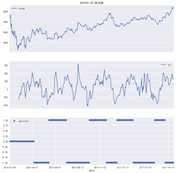
2.2 持仓信号
# 记录持仓情况,默认为0
position = 0
# 对每一交易日进行循环
for i, item in stock_index.iterrows():# 判断交易信号if item['filtered_signal'] == 1:# 交易信号为1,则记录仓位为1position = 1elif item['filtered_signal'] == -1:# 交易信号为-1, 则记录仓位为-1position = -1else:pass# 记录每日持仓情况stock_index.loc[i, 'position'] = position
stock_index.head()
plt.subplot(3, 1, 1)
plt.title('600030 CCI持仓图')
plt.gca().axes.get_xaxis().set_visible(False)
stock_index['close'].plot(figsize = (12,12))
plt.legend()
plt.subplot(3, 1, 2)
stock_index['cci'].plot(figsize = (12,12))
plt.legend()
plt.gca().axes.get_xaxis().set_visible(False)
plt.subplot(3, 1, 3)
stock_index['position'].plot(marker='o', figsize=(12,12),linestyle='')
plt.legend()
plt.show()
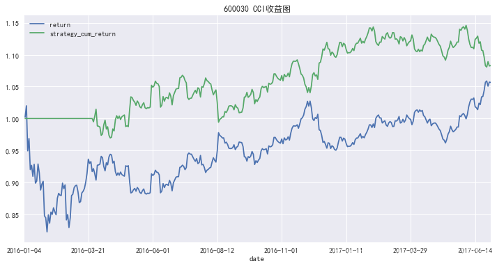
3.策略收益和数据可视化
# 计算策略收益
# 计算股票每日收益率
stock_index['pct_change'] = stock_index['close'].pct_change()
# 计算策略每日收益率
stock_index['strategy_return'] = stock_index['pct_change'] * stock_index['position']
# 计算股票累积收益率
stock_index['return'] = (stock_index['pct_change']+1).cumprod()
# 计算策略累积收益率
stock_index['strategy_cum_return'] = (1 + stock_index['strategy_return']).cumprod()
stock_index.head()
| open | close | high | low | volume | code | sma | cci | yes_close | yes_sma | ... | daybeforeyes_close | daybeforeyes_sma | sma_signal | cci_filter | filtered_signal | position | pct_change | strategy_return | return | strategy_cum_return | |
|---|---|---|---|---|---|---|---|---|---|---|---|---|---|---|---|---|---|---|---|---|---|
| date | |||||||||||||||||||||
| 2016-01-04 | 3725.86 | 3470.41 | 3726.25 | 3469.01 | 115370674.0 | hs300 | NaN | NaN | NaN | NaN | ... | NaN | NaN | 0 | 0 | 0 | 0.0 | NaN | NaN | NaN | NaN |
| 2016-01-05 | 3382.18 | 3478.78 | 3518.22 | 3377.28 | 162116984.0 | hs300 | NaN | NaN | 3470.41 | NaN | ... | NaN | NaN | 0 | 0 | 0 | 0.0 | 0.002412 | 0.0 | 1.002412 | 1.0 |
| 2016-01-06 | 3482.41 | 3539.81 | 3543.74 | 3468.47 | 145966144.0 | hs300 | NaN | NaN | 3478.78 | NaN | ... | 3470.41 | NaN | 0 | 0 | 0 | 0.0 | 0.017544 | 0.0 | 1.019998 | 1.0 |
| 2016-01-07 | 3481.15 | 3294.38 | 3481.15 | 3284.74 | 44102641.0 | hs300 | NaN | NaN | 3539.81 | NaN | ... | 3478.78 | NaN | 0 | 0 | 0 | 0.0 | -0.069334 | -0.0 | 0.949277 | 1.0 |
| 2016-01-08 | 3371.87 | 3361.56 | 3418.85 | 3237.93 | 185959451.0 | hs300 | 3428.988 | NaN | 3294.38 | NaN | ... | 3539.81 | NaN | 0 | 0 | 0 | 0.0 | 0.020392 | 0.0 | 0.968635 | 1.0 |
5 rows × 21 columns
# 将股票累积收益率和策略累积收益率绘图
stock_index[['return', 'strategy_cum_return']].plot(figsize = (12,6))plt.title('600030 CCI收益图')
plt.legend()
plt.show()
这篇关于金融量化 - 技术分析策略和交易系统_SMA+CCI交易系统的文章就介绍到这儿,希望我们推荐的文章对编程师们有所帮助!


