DeepFM代码详解及Python实现

摘要

DeepFM原理部分可以参看博客https://blog.csdn.net/weixin_45459911/article/details/105359982，本文就着重介绍其代码复现部分的内容。
本文所写的代码参考自https://www.jianshu.com/p/71d819005fed，在此基础上进行了一些修改，并增加了注释。

一、数据预处理部分

import pickle
import pandas as pd
import numpy as npdef load_data():train_data = {}file_path = '../data/tiny_train_input.csv'data = pd.read_csv(file_path, header=None)data.columns = ['c' + str(i) for i in range(data.shape[1])]  # 将列名改成了c0,c1,c2...label = data.c0.values  # 第一列label = label.reshape(len(label), 1)  # 将列向量变成行向量train_data['y_train'] = labelco_feature = pd.DataFrame()ca_feature = pd.DataFrame()ca_col = []co_col = []feat_dict = {}cnt = 1for i in range(1, data.shape[1]):target = data.iloc[:, i]  # iloc用于取出前i列col = target.name  # 得到是不包含列索引的Series结构l = len(set(target))  # set() 函数创建一个无序不重复元素集if l > 10:target = (target - target.mean()) / target.std()  # .std()函数计算标准差co_feature = pd.concat([co_feature, target], axis=1)  # 将c0_feature与target进行纵向拼接feat_dict[col] = cntcnt += 1co_col.append(col)else:us = target.unique()  # unique()是以数组形式（numpy.ndarray）返回列的所有唯一值（特征的所有唯一值）print(us)feat_dict[col] = dict(zip(us, range(cnt, len(us) + cnt)))  # zip()函数用于将可迭代的对象作为参数，将对象中对应的元素打包成一个个元组，然后返回由这些元组组成的列表ca_feature = pd.concat([ca_feature, target], axis=1)cnt += len(us)ca_col.append(col)feat_dim = cntfeature_value = pd.concat([co_feature, ca_feature], axis=1)feature_index = feature_value.copy()for i in feature_index.columns:if i in co_col:feature_index[i] = feat_dict[i]else:feature_index[i] = feature_index[i].map(feat_dict[i])feature_value[i] = 1.train_data['xi'] = feature_index.values.tolist()train_data['xv'] = feature_value.values.tolist()train_data['feat_dim'] = feat_dimreturn train_data

如上，重要的是做了两件事情，生成了feature_index和feature_value。

feature_index是把所有特征进行了标序，feature1，feature2…featurem，分别对应0，1，2，3，…m，但是，请注意分类变量需要拆分！就是说如果有性别：男|女|未知，三个选项。需要构造feature男，feature女，feature未知三个变量，而连续变量就不需要这样。

feature_value就是特征的值，连续变量按真实值填写，分类变量全部填写1。

二、DeepFM部分

1、FM部分的特征向量化

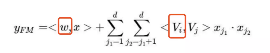
        # 特征向量化，类似原论文中的vself.weight['feature_weight'] = tf.Variable(tf.random_normal([self.feature_sizes, self.embedding_size], 0.0, 0.01),name='feature_weight')# 一次项中的w系数，类似原论文中的wself.weight['feature_first'] = tf.Variable(tf.random_normal([self.feature_sizes, 1], 0.0, 1.0),name='feature_first')

具体可参考如下公式

2、Deep部分的权重设置

        # deep网络初始input：把向量化后的特征进行拼接后带入模型，n个特征*embedding的长度input_size = self.field_size * self.embedding_sizeinit_method = np.sqrt(2.0 / (input_size + self.deep_layers[0]))self.weight['layer_0'] = tf.Variable(np.random.normal(loc=0, scale=init_method, size=(input_size, self.deep_layers[0])), dtype=np.float32)self.weight['bias_0'] = tf.Variable(np.random.normal(loc=0, scale=init_method, size=(1, self.deep_layers[0])), dtype=np.float32)# 生成deep network里面每层的weight 和 biasif num_layer != 1:for i in range(1, num_layer):init_method = np.sqrt(2.0 / (self.deep_layers[i - 1] + self.deep_layers[I]))self.weight['layer_' + str(i)] = tf.Variable(np.random.normal(loc=0, scale=init_method, size=(self.deep_layers[i - 1], self.deep_layers[i])),dtype=np.float32)self.weight['bias_' + str(i)] = tf.Variable(np.random.normal(loc=0, scale=init_method, size=(1, self.deep_layers[i])),dtype=np.float32)# deep部分output_size + 一次项output_size + 二次项output_sizelast_layer_size = self.deep_layers[-1] + self.field_size + self.embedding_sizeinit_method = np.sqrt(np.sqrt(2.0 / (last_layer_size + 1)))# 生成最后一层的结果self.weight['last_layer'] = tf.Variable(np.random.normal(loc=0, scale=init_method, size=(last_layer_size, 1)), dtype=np.float32)self.weight['last_bias'] = tf.Variable(tf.constant(0.01), dtype=np.float32)

input的地方用了个技巧，直接把把向量化后的特征进行拉伸拼接后带入模型，原来的v是batchn个特征embedding的长度，直接改成了batch*（n个特征*embedding的长度），这样的好处就是全值共享，又快又有效。

3、网络传递部分

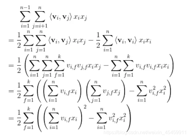
        # second_orderself.sum_second_order = tf.reduce_sum(self.embedding_part, 1)self.sum_second_order_square = tf.square(self.sum_second_order)print('sum_square_second_order:', self.sum_second_order_square)# sum_square_second_order: Tensor("Square:0", shape=(?, 256), dtype=float32)self.square_second_order = tf.square(self.embedding_part)self.square_second_order_sum = tf.reduce_sum(self.square_second_order, 1)print('square_sum_second_order:', self.square_second_order_sum)# square_sum_second_order: Tensor("Sum_2:0", shape=(?, 256), dtype=float32)# 1/2*((a+b)^2 - a^2 - b^2)=abself.second_order = 0.5 * tf.subtract(self.sum_second_order_square, self.square_second_order_sum)self.fm_part = tf.concat([self.first_order, self.second_order], axis=1)print('fm_part:', self.fm_part)

实现了下图的功能

4、loss

        # lossself.out = tf.nn.sigmoid(self.out)# loss = tf.losses.log_loss(label,out) 也行，看大家想不想自己了解一下loss的计算过程self.loss = -tf.reduce_mean(self.label * tf.log(self.out + 1e-24) + (1 - self.label) * tf.log(1 - self.out + 1e-24))# 正则：sum(w^2)/2*l2_reg_rate# 这边只加了weight，有需要的可以加上bias部分self.loss += tf.contrib.layers.l2_regularizer(self.l2_reg_rate)(self.weight["last_layer"])for i in range(len(self.deep_layers)):self.loss += tf.contrib.layers.l2_regularizer(self.l2_reg_rate)(self.weight["layer_%d" % I])

这部分重写了一下需要正则的地方，其实直接按照注释掉的部分简单操作也可以。

5、梯度正则

        self.global_step = tf.Variable(0, trainable=False)opt = tf.train.GradientDescentOptimizer(self.learning_rate)trainable_params = tf.trainable_variables()print(trainable_params)gradients = tf.gradients(self.loss, trainable_params)clip_gradients, _ = tf.clip_by_global_norm(gradients, 5)self.train_op = opt.apply_gradients(zip(clip_gradients, trainable_params), global_step=self.global_step)

很多网上的代码跑着跑着就NAN了，建议加一下梯度的正则。

6、完整代码

import numpy as np
import tensorflow as tf
import sys
from DeepFM_builddata import load_data'''
author : taowei.sha(slade sha)
time : 18.07.27
'''class Args():feature_sizes = 100field_size = 15embedding_size = 256deep_layers = [512, 256, 128]epoch = 3batch_size = 64learning_rate = 1.0l2_reg_rate = 0.01checkpoint_dir = '/Users/slade/Documents/Code/ml/data/saver/ckpt'is_training = True# deep_activation = tf.nn.reluclass model():def __init__(self, args):self.feature_sizes = args.feature_sizesself.field_size = args.field_sizeself.embedding_size = args.embedding_sizeself.deep_layers = args.deep_layersself.l2_reg_rate = args.l2_reg_rateself.epoch = args.epochself.batch_size = args.batch_sizeself.learning_rate = args.learning_rateself.deep_activation = tf.nn.reluself.weight = dict()self.checkpoint_dir = args.checkpoint_dirself.build_model()def build_model(self):self.feat_index = tf.placeholder(tf.int32, shape=[None, None], name='feature_index')self.feat_value = tf.placeholder(tf.float32, shape=[None, None], name='feature_value')self.label = tf.placeholder(tf.float32, shape=[None, None], name='label')# 特征向量化，类似原论文中的vself.weight['feature_weight'] = tf.Variable(tf.random_normal([self.feature_sizes, self.embedding_size], 0.0, 0.01),  # 生成均值为0，标准差为0.01的正态分布name='feature_weight')# 一次项中的w系数，类似原论文中的wself.weight['feature_first'] = tf.Variable(tf.random_normal([self.feature_sizes, 1], 0.0, 1.0),name='feature_first')num_layer = len(self.deep_layers)# deep网络初始input：把向量化后的特征进行拼接后带入模型，n个特征*embedding的长度input_size = self.field_size * self.embedding_sizeinit_method = np.sqrt(2.0 / (input_size + self.deep_layers[0]))self.weight['layer_0'] = tf.Variable(np.random.normal(loc=0, scale=init_method, size=(input_size, self.deep_layers[0])), dtype=np.float32)self.weight['bias_0'] = tf.Variable(np.random.normal(loc=0, scale=init_method, size=(1, self.deep_layers[0])), dtype=np.float32)# 生成deep network里面每层的weight 和 biasif num_layer != 1:for i in range(1, num_layer):init_method = np.sqrt(2.0 / (self.deep_layers[i - 1] + self.deep_layers[i]))self.weight['layer_' + str(i)] = tf.Variable(np.random.normal(loc=0, scale=init_method, size=(self.deep_layers[i - 1], self.deep_layers[i])),dtype=np.float32)self.weight['bias_' + str(i)] = tf.Variable(np.random.normal(loc=0, scale=init_method, size=(1, self.deep_layers[i])),dtype=np.float32)# deep部分output_size + 一次项output_size + 二次项output_sizelast_layer_size = self.deep_layers[-1] + self.field_size + self.embedding_sizeinit_method = np.sqrt(np.sqrt(2.0 / (last_layer_size + 1)))# 生成最后一层的结果self.weight['last_layer'] = tf.Variable(np.random.normal(loc=0, scale=init_method, size=(last_layer_size, 1)), dtype=np.float32)self.weight['last_bias'] = tf.Variable(tf.constant(0.01), dtype=np.float32)# embedding_partself.embedding_index = tf.nn.embedding_lookup(self.weight['feature_weight'],self.feat_index)  # Batch*F*Kself.embedding_part = tf.multiply(self.embedding_index,tf.reshape(self.feat_value, [-1, self.field_size, 1]))# [Batch*F*1] * [Batch*F*K] = [Batch*F*K],用到了broadcast的属性print('embedding_part:', self.embedding_part)# embedding_part: Tensor("Mul:0", shape=(?, 15, 256), dtype=float32)# first_orderself.embedding_first = tf.nn.embedding_lookup(self.weight['feature_first'],self.feat_index)  # bacth*F*1self.embedding_first = tf.multiply(self.embedding_first, tf.reshape(self.feat_value, [-1, self.field_size, 1]))self.first_order = tf.reduce_sum(self.embedding_first, 2)print('first_order:', self.first_order)# first_order: Tensor("Sum:0", shape=(?, 15), dtype=float32)# second_orderself.sum_second_order = tf.reduce_sum(self.embedding_part, 1)self.sum_second_order_square = tf.square(self.sum_second_order)print('sum_square_second_order:', self.sum_second_order_square)# sum_square_second_order: Tensor("Square:0", shape=(?, 256), dtype=float32)self.square_second_order = tf.square(self.embedding_part)self.square_second_order_sum = tf.reduce_sum(self.square_second_order, 1)print('square_sum_second_order:', self.square_second_order_sum)# square_sum_second_order: Tensor("Sum_2:0", shape=(?, 256), dtype=float32)# 1/2*((a+b)^2 - a^2 - b^2)=abself.second_order = 0.5 * tf.subtract(self.sum_second_order_square, self.square_second_order_sum)self.fm_part = tf.concat([self.first_order, self.second_order], axis=1)print('fm_part:', self.fm_part)# fm_part: Tensor("concat:0", shape=(?, 271), dtype=float32)# deep partself.deep_embedding = tf.reshape(self.embedding_part, [-1, self.field_size * self.embedding_size])print('deep_embedding:', self.deep_embedding)for i in range(0, len(self.deep_layers)):self.deep_embedding = tf.add(tf.matmul(self.deep_embedding, self.weight["layer_%d" % i]),self.weight["bias_%d" % i])self.deep_embedding = self.deep_activation(self.deep_embedding)# concatdin_all = tf.concat([self.fm_part, self.deep_embedding], axis=1)self.out = tf.add(tf.matmul(din_all, self.weight['last_layer']), self.weight['last_bias'])print('outputs:', self.out)# lossself.out = tf.nn.sigmoid(self.out)# loss = tf.losses.log_loss(label,out) 也行，看大家想不想自己了解一下loss的计算过程self.loss = -tf.reduce_mean(self.label * tf.log(self.out + 1e-24) + (1 - self.label) * tf.log(1 - self.out + 1e-24))# 正则：sum(w^2)/2*l2_reg_rate# 这边只加了weight，有需要的可以加上bias部分self.loss += tf.contrib.layers.l2_regularizer(self.l2_reg_rate)(self.weight["last_layer"])for i in range(len(self.deep_layers)):self.loss += tf.contrib.layers.l2_regularizer(self.l2_reg_rate)(self.weight["layer_%d" % i])self.global_step = tf.Variable(0, trainable=False)opt = tf.train.GradientDescentOptimizer(self.learning_rate)trainable_params = tf.trainable_variables()print(trainable_params)gradients = tf.gradients(self.loss, trainable_params)clip_gradients, _ = tf.clip_by_global_norm(gradients, 5)self.train_op = opt.apply_gradients(zip(clip_gradients, trainable_params), global_step=self.global_step)def train(self, sess, feat_index, feat_value, label):loss, _, step = sess.run([self.loss, self.train_op, self.global_step], feed_dict={self.feat_index: feat_index,self.feat_value: feat_value,self.label: label})return loss, stepdef predict(self, sess, feat_index, feat_value):result = sess.run([self.out], feed_dict={self.feat_index: feat_index,self.feat_value: feat_value})return resultdef save(self, sess, path):saver = tf.train.Saver()saver.save(sess, save_path=path)def restore(self, sess, path):saver = tf.train.Saver()saver.restore(sess, save_path=path)def get_batch(Xi, Xv, y, batch_size, index):start = index * batch_sizeend = (index + 1) * batch_sizeend = end if end < len(y) else len(y)return Xi[start:end], Xv[start:end], np.array(y[start:end])if __name__ == '__main__':args = Args()gpu_config = tf.ConfigProto()gpu_config.gpu_options.allow_growth = Truedata = load_data()args.feature_sizes = data['feat_dim']args.field_size = len(data['xi'][0])args.is_training = Truewith tf.Session(config=gpu_config) as sess:Model = model(args)# init variablessess.run(tf.global_variables_initializer())sess.run(tf.local_variables_initializer())cnt = int(len(data['y_train']) / args.batch_size)print('time all:%s' % cnt)sys.stdout.flush()if args.is_training:for i in range(args.epoch):print('epoch %s:' % i)for j in range(0, cnt):X_index, X_value, y = get_batch(data['xi'], data['xv'], data['y_train'], args.batch_size, j)loss, step = Model.train(sess, X_index, X_value, y)if j % 100 == 0:print('the times of training is %d, and the loss is %s' % (j, loss))Model.save(sess, args.checkpoint_dir)else:Model.restore(sess, args.checkpoint_dir)for j in range(0, cnt):X_index, X_value, y = get_batch(data['xi'], data['xv'], data['y_train'], args.batch_size, j)result = Model.predict(sess, X_index, X_value)print(result)

三、执行结果和测试数据集

执行结果

/Users/slade/anaconda3/bin/python /Users/slade/Documents/Personalcode/machine-learning/Python/deepfm/deepfm.py
[2 1 0 3 4 6 5 7]
[0 1 2]
[6 0 8 2 4 1 7 3 5 9]
[2 3 1 0]
W tensorflow/core/platform/cpu_feature_guard.cc:45] The TensorFlow library wasn't compiled to use SSE4.1 instructions, but these are available on your machine and could speed up CPU computations.
W tensorflow/core/platform/cpu_feature_guard.cc:45] The TensorFlow library wasn't compiled to use SSE4.2 instructions, but these are available on your machine and could speed up CPU computations.
W tensorflow/core/platform/cpu_feature_guard.cc:45] The TensorFlow library wasn't compiled to use AVX instructions, but these are available on your machine and could speed up CPU computations.
W tensorflow/core/platform/cpu_feature_guard.cc:45] The TensorFlow library wasn't compiled to use AVX2 instructions, but these are available on your machine and could speed up CPU computations.
W tensorflow/core/platform/cpu_feature_guard.cc:45] The TensorFlow library wasn't compiled to use FMA instructions, but these are available on your machine and could speed up CPU computations.
embedding_part: Tensor("Mul:0", shape=(?, 39, 256), dtype=float32)
first_order: Tensor("Sum:0", shape=(?, 39), dtype=float32)
sum_square_second_order: Tensor("Square:0", shape=(?, 256), dtype=float32)
square_sum_second_order: Tensor("Sum_2:0", shape=(?, 256), dtype=float32)
fm_part: Tensor("concat:0", shape=(?, 295), dtype=float32)
deep_embedding: Tensor("Reshape_2:0", shape=(?, 9984), dtype=float32)
output: Tensor("Add_3:0", shape=(?, 1), dtype=float32)
[<tensorflow.python.ops.variables.Variable object at 0x10e2a9ba8>, <tensorflow.python.ops.variables.Variable object at 0x112885ef0>, <tensorflow.python.ops.variables.Variable object at 0x1129b3c18>, <tensorflow.python.ops.variables.Variable object at 0x1129b3da0>, <tensorflow.python.ops.variables.Variable object at 0x1129b3f28>, <tensorflow.python.ops.variables.Variable object at 0x1129b3c50>, <tensorflow.python.ops.variables.Variable object at 0x112a03dd8>, <tensorflow.python.ops.variables.Variable object at 0x112a03b38>, <tensorflow.python.ops.variables.Variable object at 0x16eae5c88>, <tensorflow.python.ops.variables.Variable object at 0x112b937b8>]
time all:7156
epoch 0:
the times of training is 0, and the loss is 8.54514
the times of training is 100, and the loss is 1.60875
the times of training is 200, and the loss is 0.681524
the times of training is 300, and the loss is 0.617403
the times of training is 400, and the loss is 0.431383
the times of training is 500, and the loss is 0.531491
the times of training is 600, and the loss is 0.558392
the times of training is 800, and the loss is 0.51909
...

测试数据集
可以点击这里下载，我设置了0积分。
https://download.csdn.net/download/weixin_45459911/12326542

参考：https://www.jianshu.com/p/71d819005fed