2.9-tf2-数据增强-tf_flowers

1.导入包

import matplotlib.pyplot as plt
import numpy as np
import tensorflow as tf
import tensorflow_datasets as tfdsfrom tensorflow.keras import layers
from tensorflow.keras.datasets import mnist

2.加载数据

(train_ds, val_ds, test_ds), metadata = tfds.load('tf_flowers',split=['train[:80%]', 'train[80%:90%]', 'train[90%:]'],with_info=True,as_supervised=True,
)

#The flowers dataset has five classes.num_classes = metadata.features['label'].num_classes
print(num_classes)
5

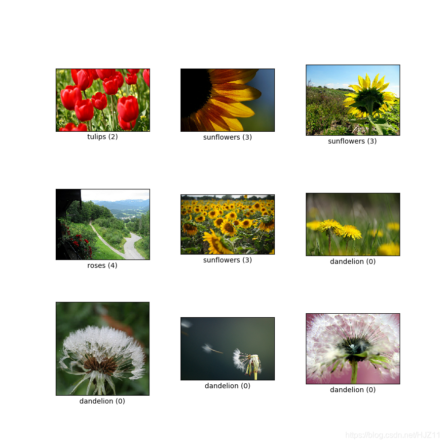
复现数据:

#Let's retrieve an image from the dataset and use it to demonstrate data augmentation.get_label_name = metadata.features['label'].int2strimage, label = next(iter(train_ds))
_ = plt.imshow(image)
_ = plt.title(get_label_name(label))

3.数据预处理

Use Keras preprocessing layers

#Resizing and rescaling
#You can use preprocessing layers to resize your images to a consistent shape, and to rescale pixel values.IMG_SIZE = 180resize_and_rescale = tf.keras.Sequential([layers.experimental.preprocessing.Resizing(IMG_SIZE, IMG_SIZE),layers.experimental.preprocessing.Rescaling(1./255)
])
#Note: the rescaling layer above standardizes pixel values to [0,1]. If instead you wanted [-1,1], you would write Rescaling(1./127.5, offset=-1).

result = resize_and_rescale(image)
_ = plt.imshow(result)

#You can verify the pixels are in [0-1].print("Min and max pixel values:", result.numpy().min(), result.numpy().max())

Min and max pixel values: 0.0 1.0

4.数据增强

#Data augmentation
#You can use preprocessing layers for data augmentation as well.#Let's create a few preprocessing layers and apply them repeatedly to the same image.data_augmentation = tf.keras.Sequential([layers.experimental.preprocessing.RandomFlip("horizontal_and_vertical"),layers.experimental.preprocessing.RandomRotation(0.2),
])

# Add the image to a batch
image = tf.expand_dims(image, 0)

plt.figure(figsize=(10, 10))
for i in range(9):augmented_image = data_augmentation(image)ax = plt.subplot(3, 3, i + 1)plt.imshow(augmented_image[0])plt.axis("off")

#There are a variety of preprocessing layers you can use for data augmentation including layers.RandomContrast, layers.RandomCrop, layers.RandomZoom, and others.

5.预处理层的两种方法

There are two ways you can use these preprocessing layers, with important tradeoffs.

1. 第一种方法

Option 1: Make the preprocessing layers part of your model
model = tf.keras.Sequential([resize_and_rescale,data_augmentation,layers.Conv2D(16, 3, padding='same', activation='relu'),layers.MaxPooling2D(),# Rest of your model
])

There are two important points to be aware of in this case:Data augmentation will run on-device, synchronously with the rest of your layers, and benefit from GPU acceleration.When you export your model using model.save, the preprocessing layers will be saved along with the rest of your model. If you later deploy this model, it will automatically standardize images (according to the configuration of your layers). This can save you from the effort of having to reimplement that logic server-side.Note: Data augmentation is inactive at test time so input images will only be augmented during calls to model.fit (not model.evaluate or model.predict).

2. 第二种方法:

#Option 2: Apply the preprocessing layers to your dataset
aug_ds = train_ds.map(lambda x, y: (resize_and_rescale(x, training=True), y))

With this approach, you use Dataset.map to create a dataset that yields batches of augmented images. In this case:Data augmentation will happen asynchronously on the CPU, and is non-blocking. You can overlap the training of your model on the GPU with data preprocessing, using Dataset.prefetch, shown below.
In this case the prepreprocessing layers will not be exported with the model when you call model.save. You will need to attach them to your model before saving it or reimplement them server-side. After training, you can attach the preprocessing layers before export.

6.把与处理层用在数据集上

Configure the train, validation, and test datasets with the preprocessing layers you created above. You will also configure the datasets for performance, using parallel reads and buffered prefetching to yield batches from disk without I/O become blocking. 

Note: data augmentation should only be applied to the training set.

batch_size = 32
AUTOTUNE = tf.data.experimental.AUTOTUNEdef prepare(ds, shuffle=False, augment=False):# Resize and rescale all datasetsds = ds.map(lambda x, y: (resize_and_rescale(x), y), num_parallel_calls=AUTOTUNE)if shuffle:ds = ds.shuffle(1000)# Batch all datasetsds = ds.batch(batch_size)# Use data augmentation only on the training setif augment:ds = ds.map(lambda x, y: (data_augmentation(x, training=True), y), num_parallel_calls=AUTOTUNE)# Use buffered prefecting on all datasetsreturn ds.prefetch(buffer_size=AUTOTUNE)

train_ds = prepare(train_ds, shuffle=True, augment=True)
val_ds = prepare(val_ds)
test_ds = prepare(test_ds)

7.训练模型

model = tf.keras.Sequential([layers.Conv2D(16, 3, padding='same', activation='relu'),layers.MaxPooling2D(),layers.Conv2D(32, 3, padding='same', activation='relu'),layers.MaxPooling2D(),layers.Conv2D(64, 3, padding='same', activation='relu'),layers.MaxPooling2D(),layers.Flatten(),layers.Dense(128, activation='relu'),layers.Dense(num_classes)
])

model.compile(optimizer='adam',loss=tf.keras.losses.SparseCategoricalCrossentropy(from_logits=True),metrics=['accuracy'])

epochs=5
history = model.fit(train_ds,validation_data=val_ds,epochs=epochs
)

Epoch 1/5
92/92 [==============================] - 30s 315ms/step - loss: 1.5078 - accuracy: 0.3428 - val_loss: 1.0809 - val_accuracy: 0.6240
Epoch 2/5
92/92 [==============================] - 28s 303ms/step - loss: 1.0781 - accuracy: 0.5724 - val_loss: 0.9762 - val_accuracy: 0.6322
Epoch 3/5
92/92 [==============================] - 28s 295ms/step - loss: 1.0083 - accuracy: 0.5900 - val_loss: 0.9570 - val_accuracy: 0.6376
Epoch 4/5
92/92 [==============================] - 28s 300ms/step - loss: 0.9537 - accuracy: 0.6116 - val_loss: 0.9081 - val_accuracy: 0.6485
Epoch 5/5
92/92 [==============================] - 28s 301ms/step - loss: 0.8816 - accuracy: 0.6525 - val_loss: 0.8353 - val_accuracy: 0.6594

loss, acc = model.evaluate(test_ds)
print("Accuracy", acc)

12/12 [==============================] - 1s 83ms/step - loss: 0.8226 - accuracy: 0.6567
Accuracy 0.6566757559776306

8.自定义数据增强

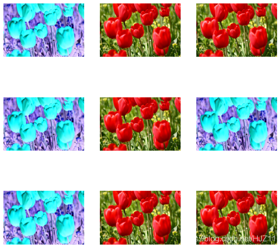
First, you will create a layers.Lambda layer. This is a good way to write concise code. Next, you will write a new layer via subclassing, which gives you more control. Both layers will randomly invert the colors in an image, accoring to some probability.

def random_invert_img(x, p=0.5):if  tf.random.uniform([]) < p:x = (255-x)else:xreturn xdef random_invert(factor=0.5):return layers.Lambda(lambda x: random_invert_img(x, factor))random_invert = random_invert()plt.figure(figsize=(10, 10))
for i in range(9):augmented_image = random_invert(image)ax = plt.subplot(3, 3, i + 1)plt.imshow(augmented_image[0].numpy().astype("uint8"))plt.axis("off")

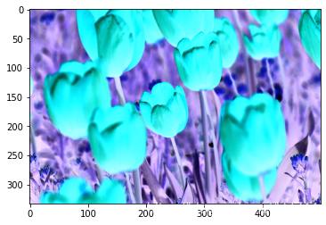
#Next, implement a custom layer by subclassing.class RandomInvert(layers.Layer):def __init__(self, factor=0.5, **kwargs):super().__init__(**kwargs)self.factor = factordef call(self, x):return random_invert_img(x)_ = plt.imshow(RandomInvert()(image)[0])

9.Using tf.image

Since the flowers dataset was previously configured with data augmentation, let's reimport it to start fresh.(train_ds, val_ds, test_ds), metadata = tfds.load('tf_flowers',split=['train[:80%]', 'train[80%:90%]', 'train[90%:]'],with_info=True,as_supervised=True,
)

#Retrieve an image to work with.image, label = next(iter(train_ds))
_ = plt.imshow(image)
_ = plt.title(get_label_name(label))

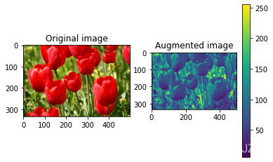
Let's use the following function to visualize and compare the original and augmented images side-by-side.def visualize(original, augmented):fig = plt.figure()plt.subplot(1,2,1)plt.title('Original image')plt.imshow(original)plt.subplot(1,2,2)plt.title('Augmented image')plt.imshow(augmented)

#Data augmentation
#Flipping the image
3Flip the image either vertically or horizontally.flipped = tf.image.flip_left_right(image)
visualize(image, flipped)

#Grayscale an image.grayscaled = tf.image.rgb_to_grayscale(image)
visualize(image, tf.squeeze(grayscaled))
_ = plt.colorbar()

#Saturate an image by providing a saturation factor.saturated = tf.image.adjust_saturation(image, 3)
visualize(image, saturated)

#Change image brightness
#Change the brightness of image by providing a brightness factor.bright = tf.image.adjust_brightness(image, 0.4)
visualize(image, bright)

#Center crop the image
#Crop the image from center up to the image part you desire.cropped = tf.image.central_crop(image, central_fraction=0.5)
visualize(image,cropped)

#Rotate the image
#Rotate an image by 90 degrees.rotated = tf.image.rot90(image)
visualize(image, rotated)

#Apply augmentation to a dataset
#As before, apply data augmentation to a dataset using Dataset.map.def resize_and_rescale(image, label):image = tf.cast(image, tf.float32)image = tf.image.resize(image, [IMG_SIZE, IMG_SIZE])image = (image / 255.0)return image, labeldef augment(image,label):image, label = resize_and_rescale(image, label)# Add 6 pixels of paddingimage = tf.image.resize_with_crop_or_pad(image, IMG_SIZE + 6, IMG_SIZE + 6) # Random crop back to the original sizeimage = tf.image.random_crop(image, size=[IMG_SIZE, IMG_SIZE, 3])image = tf.image.random_brightness(image, max_delta=0.5) # Random brightnessimage = tf.clip_by_value(image, 0, 1)return image, label

#Configure the datasets
train_ds = (train_ds.shuffle(1000).map(augment, num_parallel_calls=AUTOTUNE).batch(batch_size).prefetch(AUTOTUNE)
) val_ds = (val_ds.map(resize_and_rescale, num_parallel_calls=AUTOTUNE).batch(batch_size).prefetch(AUTOTUNE)
)test_ds = (test_ds.map(resize_and_rescale, num_parallel_calls=AUTOTUNE).batch(batch_size).prefetch(AUTOTUNE)
)#These datasets can now be used to train a model as shown previously.