本文主要是介绍python中正弦函数模块_python3 的matplotlib的4种办法制作动态sin函数程序详述,希望对大家解决编程问题提供一定的参考价值,需要的开发者们随着小编来一起学习吧!
1.说明:
1.1 推荐指数:★★★
1.2 python的基础知识复习,通过生动的sin函数制作来复习return和yield,列表、函数定义等知识。
1.3 熟悉matplotlib作图相关知识。
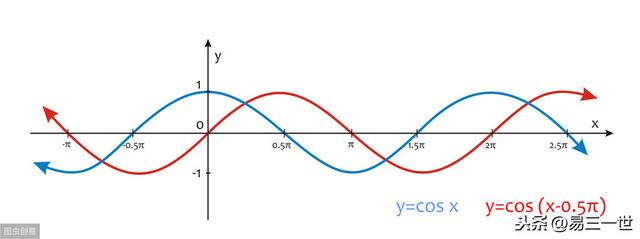
1.4 加深理解sin函数,为以后圆的理解打下坚实基础,cos重复不解释了,将sin适当修改即可。
2.return法,基本方法,代码:
#---导出模块---
import numpy as np
from matplotlib import pyplot as plt
from matplotlib import animation
#定义画布,默认值,这个fig需要,虽然默认大小设置,fig需要挂在动画上
fig = plt.figure()
#坐标轴刻度
ax = plt.axes(xlim=(0, 2), ylim=(-2, 2))
#color='blue'=蓝色,否则默认为清淡蓝色
line, = ax.plot([], [], lw=2,color='blue')
# 因为动画,所以初始化列表线条
def init():
line.set_data([], [])
return line, #注意逗号
#定义动画
def animate(i):
#x取值范围从0~2,等差数列,分成1000,越大线条越平滑
x = np.linspace(0, 2, 1000)
#动画x和y的值与i的从0~i的取值有关,才动起来
y = np.sin(2 * np.pi * (x - 0.01 * i))
line.set_data(x, y)
return line, #注意逗号
#将fig挂在动画上面
anim = animation.FuncAnimation(fig, animate, init_func=init,frames=200, interval=20, blit=True)
#如果需要保存动画,就这样
#anim.save('basic_animation.mp4', fps=30, extra_args=['-vcodec', 'libx264'])
#标题名称
plt.title('Sin-a-subplot')
plt.show()
图1
3.np.nan法,代码:
#---导出模块---
import numpy as np
import matplotlib.pyplot as plt
import matplotlib.animation as animation
#---定义画布---重点讲到区别和含义---
fig, ax = plt.subplots()
#---函数定义法---讲的很清楚了,很多遍---
#复习一下
#x的坐标取值范围,arange法一般是-2π到2π,这里是从0取,0.01,数值越小曲线越平滑
#注意与linspace取等差数列的区别
x = np.arange(0, 2*np.pi, 0.01)
#这是一步并2步了,相当于y=np.sin(x)
line, = ax.plot(x, np.sin(x))
#---初始化---注意np.nan(NaN)知识复习---
def init():
line.set_ydata([np.nan] * len(x))
#等同于下面
#line.set_ydata([] * len(x))
return line,
'''
有两种丢失数据:
None
np.nan(NaN)
None是Python自带的,其类型为python object。因此,None不能参与到任何计算中。
np.nan(NaN)
np.nan是浮点类型,能参与到计算中。但计算的结果总是NaN。
但可以使用np.nan*()函数来计算nan,此时视nan为0。
'''
#---定义动画---
def animate(i):
#line.set_ydata(np.sin(x + i / 100))
#与上面一样效果
line.set_ydata(np.sin(x + 0.01 * i))
return line,
#fig的挂在动画上面
ani = animation.FuncAnimation(fig, animate, init_func=init, interval=2, blit=True, save_count=50)
# ani.save("movie.mp4")
plt.show()
图2
4.带红色小圆点的yield法,代码:
#---导出模块---
import numpy as np
import matplotlib.pyplot as plt
from matplotlib import animation
#---定义画布和ax轴---
fig, ax = plt.subplots()
'''
等价于:fig, ax = plt.subplots(11)=fig, ax = plt.subplots(1,1)
=fig, ax1 = plt.subplot()
或者:
fig = plt.figure()
ax = fig.add_subplot(1,1,1)
'''
#---x和y的函数关系---
x = np.linspace(0, 2*np.pi, 200)
y = np.sin(x)
#画正弦函数线
l = ax.plot(x, y)
#运动的圆球,ro=就是red的o=红色的圆球,如果是o,就是默认颜色的圆球
#挂在正弦函数线上的球,初始化坐标为空
dot, = ax.plot([], [], 'ro')
#---初始化定义红色圆球的ax坐标取值范围---
def init():
ax.set_xlim(0, 2*np.pi)
ax.set_ylim(-1, 1)
return l
#---产生圆球的坐标取值范围,符合正弦函数---
def gen_dot():
#i类似x坐标,np.sin(i)类似y坐标
for i in np.linspace(0, 2*np.pi, 200):
newdot = [i, np.sin(i)]
#通过yield函数产生
yield newdot
'''
首先比较下return 与 yield的区别:
return:在程序函数中返回某个值,返回之后函数不在继续执行,彻底结束。
yield: 带有yield的函数是一个迭代器,函数返回某个值时,会停留在某个位置,返回函数值后,会在前面停留的位置继续执行,直到程序结束
带有 yield 的函数不再是一个普通函数,而是一个生成器generator,可用于迭代。
'''
#---更新小圆球的位置---
def update_dot(newd):
dot.set_data(newd[0], newd[1])
return dot,
#---定义动画---
ani = animation.FuncAnimation(fig, update_dot, frames = gen_dot, interval = 100, init_func=init)
#ani.save('sin_dot.gif', writer='imagemagick', fps=30)
plt.show()
图3
5 timer法:最新matplotlib好像淘汰了,可以运行,但是报错,可以不用管它,学习技术而已。代码如下:
#---导出模块---
import matplotlib.pyplot as plt
import numpy as np
#---fig和ax放在一起
fig, ax = plt.subplots()
#---初始化定义---
points_dot = 100
#复习一下列表知识,一个列表里有100个相同的0的列表
sin_list = [0] * points_dot
indx = 0
#---画正弦函数线---初始化---
line_sin, = ax.plot(range(points_dot), sin_list, label='sin-d', color='blue')
#---定义sin输出函数---
def sin_output(ax):
global indx, sin_list, line_sin
if indx == 20:
indx = 0
indx += 1
#更新sin列表,初始化全是100个0,更新后就是正弦函数的y坐标
sin_list = sin_list[1:] + [np.sin((indx / 10) * np.pi)]
#看看ydata就是y坐标的意思
line_sin.set_ydata(sin_list)
#从新画正弦函数动态曲线
ax.draw_artist(line_sin)
ax.figure.canvas.draw()
#计时器在新版的matplotlib中已经删除,目前能显示,但是报错,可以不管,暂时学学技术,了解一下
timer = fig.canvas.new_timer(interval=100)
timer.add_callback(sin_output, ax)
timer.start()
#x和y轴的刻度定义
ax.set_xlim([0, points_dot])
ax.set_ylim([-2, 2])
#ax.set_autoscale_on(False) #默认False
#0~100,每隔10取刻度值
ax.set_xticks(range(0, points_dot, 10))
ax.set_yticks(range(-2, 3, 1))
#显示网格
ax.grid(True)
#显示图例,固定位置=中心上面
ax.legend(loc='upper center', ncol=4)
plt.show()
'''
报错:
RuntimeError: wrapped C/C++ object of type QTimer has been deleted
提示新版的matplotlib已经删除timer了
'''
图4
希望喜欢,收藏之后好好复习,生动的图像,加深对python的基础知识的理解,熟悉matplotlib作图,以后拿来就用,通俗易懂。感谢作者分享-http://bjbsair.com/2020-04-07/tech-info/30776.html
1.说明:
1.1 推荐指数:★★★
1.2 python的基础知识复习,通过生动的sin函数制作来复习return和yield,列表、函数定义等知识。
1.3 熟悉matplotlib作图相关知识。
1.4 加深理解sin函数,为以后圆的理解打下坚实基础,cos重复不解释了,将sin适当修改即可。
2.return法,基本方法,代码:
#---导出模块---
import numpy as np
from matplotlib import pyplot as plt
from matplotlib import animation
#定义画布,默认值,这个fig需要,虽然默认大小设置,fig需要挂在动画上
fig = plt.figure()
#坐标轴刻度
ax = plt.axes(xlim=(0, 2), ylim=(-2, 2))
#color='blue'=蓝色,否则默认为清淡蓝色
line, = ax.plot([], [], lw=2,color='blue')
# 因为动画,所以初始化列表线条
def init():
line.set_data([], [])
return line, #注意逗号
#定义动画
def animate(i):
#x取值范围从0~2,等差数列,分成1000,越大线条越平滑
x = np.linspace(0, 2, 1000)
#动画x和y的值与i的从0~i的取值有关,才动起来
y = np.sin(2 * np.pi * (x - 0.01 * i))
line.set_data(x, y)
return line, #注意逗号
#将fig挂在动画上面
anim = animation.FuncAnimation(fig, animate, init_func=init,frames=200, interval=20, blit=True)
#如果需要保存动画,就这样
#anim.save('basic_animation.mp4', fps=30, extra_args=['-vcodec', 'libx264'])
#标题名称
plt.title('Sin-a-subplot')
plt.show()
图1
3.np.nan法,代码:
#---导出模块---
import numpy as np
import matplotlib.pyplot as plt
import matplotlib.animation as animation
#---定义画布---重点讲到区别和含义---
fig, ax = plt.subplots()
#---函数定义法---讲的很清楚了,很多遍---
#复习一下
#x的坐标取值范围,arange法一般是-2π到2π,这里是从0取,0.01,数值越小曲线越平滑
#注意与linspace取等差数列的区别
x = np.arange(0, 2*np.pi, 0.01)
#这是一步并2步了,相当于y=np.sin(x)
line, = ax.plot(x, np.sin(x))
#---初始化---注意np.nan(NaN)知识复习---
def init():
line.set_ydata([np.nan] * len(x))
#等同于下面
#line.set_ydata([] * len(x))
return line,
'''
有两种丢失数据:
None
np.nan(NaN)
None是Python自带的,其类型为python object。因此,None不能参与到任何计算中。
np.nan(NaN)
np.nan是浮点类型,能参与到计算中。但计算的结果总是NaN。
但可以使用np.nan*()函数来计算nan,此时视nan为0。
'''
#---定义动画---
def animate(i):
#line.set_ydata(np.sin(x + i / 100))
#与上面一样效果
line.set_ydata(np.sin(x + 0.01 * i))
return line,
#fig的挂在动画上面
ani = animation.FuncAnimation(fig, animate, init_func=init, interval=2, blit=True, save_count=50)
# ani.save("movie.mp4")
plt.show()
图2
4.带红色小圆点的yield法,代码:
#---导出模块---
import numpy as np
import matplotlib.pyplot as plt
from matplotlib import animation
#---定义画布和ax轴---
fig, ax = plt.subplots()
'''
等价于:fig, ax = plt.subplots(11)=fig, ax = plt.subplots(1,1)
=fig, ax1 = plt.subplot()
或者:
fig = plt.figure()
ax = fig.add_subplot(1,1,1)
'''
#---x和y的函数关系---
x = np.linspace(0, 2*np.pi, 200)
y = np.sin(x)
#画正弦函数线
l = ax.plot(x, y)
#运动的圆球,ro=就是red的o=红色的圆球,如果是o,就是默认颜色的圆球
#挂在正弦函数线上的球,初始化坐标为空
dot, = ax.plot([], [], 'ro')
#---初始化定义红色圆球的ax坐标取值范围---
def init():
ax.set_xlim(0, 2*np.pi)
ax.set_ylim(-1, 1)
return l
#---产生圆球的坐标取值范围,符合正弦函数---
def gen_dot():
#i类似x坐标,np.sin(i)类似y坐标
for i in np.linspace(0, 2*np.pi, 200):
newdot = [i, np.sin(i)]
#通过yield函数产生
yield newdot
'''
首先比较下return 与 yield的区别:
return:在程序函数中返回某个值,返回之后函数不在继续执行,彻底结束。
yield: 带有yield的函数是一个迭代器,函数返回某个值时,会停留在某个位置,返回函数值后,会在前面停留的位置继续执行,直到程序结束
带有 yield 的函数不再是一个普通函数,而是一个生成器generator,可用于迭代。
'''
#---更新小圆球的位置---
def update_dot(newd):
dot.set_data(newd[0], newd[1])
return dot,
#---定义动画---
ani = animation.FuncAnimation(fig, update_dot, frames = gen_dot, interval = 100, init_func=init)
#ani.save('sin_dot.gif', writer='imagemagick', fps=30)
plt.show()
图3
5 timer法:最新matplotlib好像淘汰了,可以运行,但是报错,可以不用管它,学习技术而已。代码如下:
#---导出模块---
import matplotlib.pyplot as plt
import numpy as np
#---fig和ax放在一起
fig, ax = plt.subplots()
#---初始化定义---
points_dot = 100
#复习一下列表知识,一个列表里有100个相同的0的列表
sin_list = [0] * points_dot
indx = 0
#---画正弦函数线---初始化---
line_sin, = ax.plot(range(points_dot), sin_list, label='sin-d', color='blue')
#---定义sin输出函数---
def sin_output(ax):
global indx, sin_list, line_sin
if indx == 20:
indx = 0
indx += 1
#更新sin列表,初始化全是100个0,更新后就是正弦函数的y坐标
sin_list = sin_list[1:] + [np.sin((indx / 10) * np.pi)]
#看看ydata就是y坐标的意思
line_sin.set_ydata(sin_list)
#从新画正弦函数动态曲线
ax.draw_artist(line_sin)
ax.figure.canvas.draw()
#计时器在新版的matplotlib中已经删除,目前能显示,但是报错,可以不管,暂时学学技术,了解一下
timer = fig.canvas.new_timer(interval=100)
timer.add_callback(sin_output, ax)
timer.start()
#x和y轴的刻度定义
ax.set_xlim([0, points_dot])
ax.set_ylim([-2, 2])
#ax.set_autoscale_on(False) #默认False
#0~100,每隔10取刻度值
ax.set_xticks(range(0, points_dot, 10))
ax.set_yticks(range(-2, 3, 1))
#显示网格
ax.grid(True)
#显示图例,固定位置=中心上面
ax.legend(loc='upper center', ncol=4)
plt.show()
'''
报错:
RuntimeError: wrapped C/C++ object of type QTimer has been deleted
提示新版的matplotlib已经删除timer了
'''
图4
希望喜欢,收藏之后好好复习,生动的图像,加深对python的基础知识的理解,熟悉matplotlib作图,以后拿来就用,通俗易懂。
这篇关于python中正弦函数模块_python3 的matplotlib的4种办法制作动态sin函数程序详述的文章就介绍到这儿,希望我们推荐的文章对编程师们有所帮助!


