随机森林应用案例 —— otto产品分类

1 案例背景

奥托集团是世界上最大的电子商务公司之一，在20多个国家设有子公司。该公司每天都在世界各地销售数百万种产品,所以对其产品根据性能合理的分类非常重要。

不过,在实际工作中,工作人员发现,许多相同的产品得到了不同的分类。本案例要求,你对奥拓集团的产品进行正确的分类。尽可能的提供分类的准确性。

2 数据集介绍

本案例中，数据集包含大约200,000种产品的93个特征。其目的是建立一个能够区分otto公司主要产品类别的预测模型。所有产品共被分成九个类别（例如时装，电子产品等）

• id - 产品id
• feat_1, feat_2, …, feat_93 - 产品的各个特征
• target - 产品被划分的类别

数据集：https://www.kaggle.com/c/otto-group-product-classification-challenge/overview

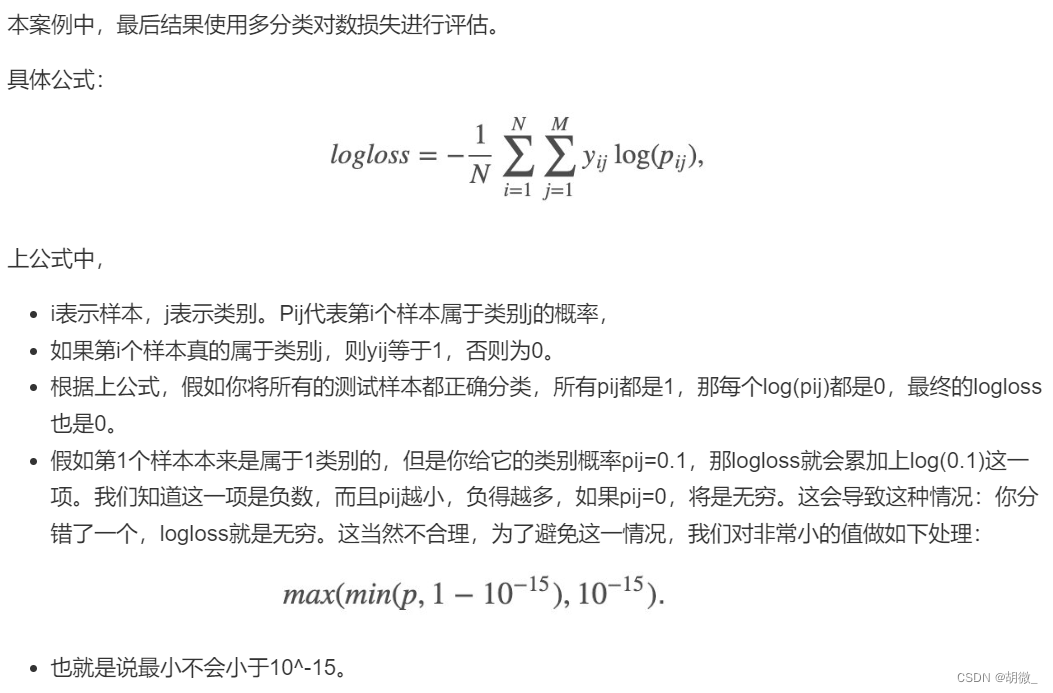
3 评分标准

4 流程实现

4.1 获取数据集

import pandas as pd
import numpy as np
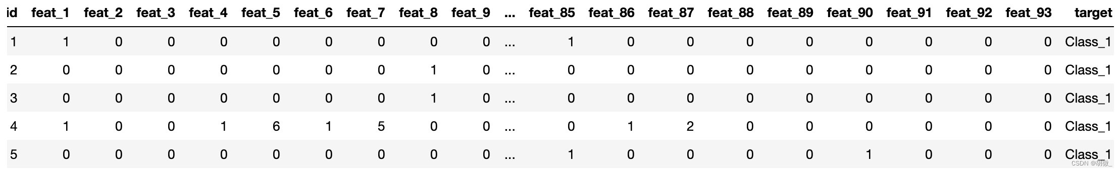
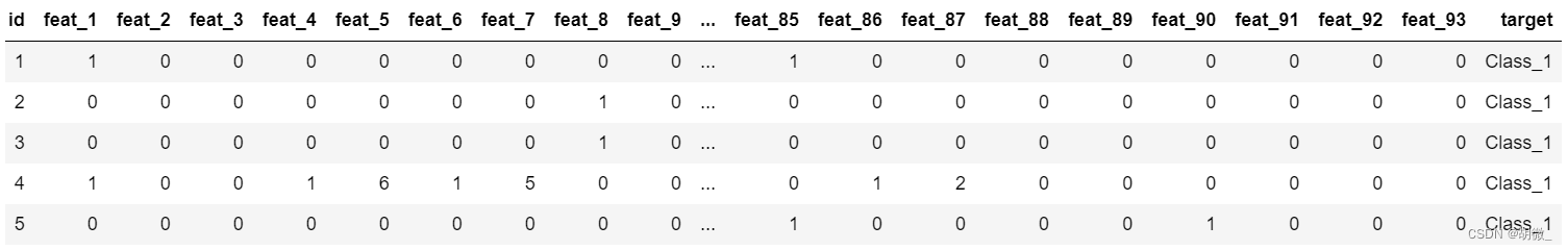
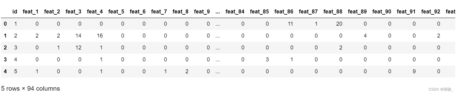
import matplotlib.pyplot as pltdata = pd.read_csv("./Data/otto/train.csv")
data.head()

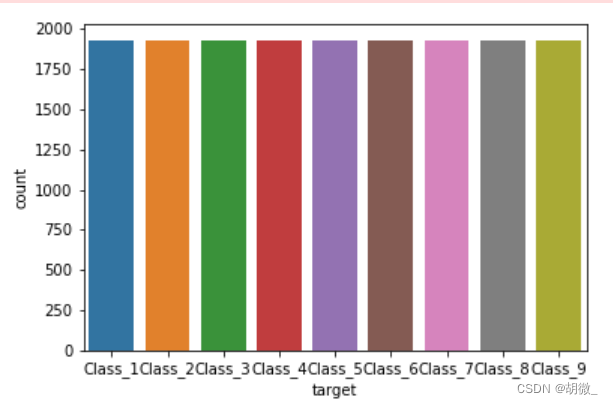
查看数据分布

import seaborn as snssns.countplot(data.target)
plt.show()

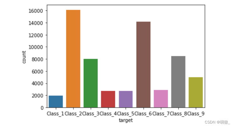
由上图可以看出，该数据类别不均衡，因数据量庞大，采用随机欠采样进行处理

4.2 数据基本处理

（1）确定特征值和标签值

# 采用随机欠采样之前需要确定数据的特征值和标签值
y=data["target"]
x=data.drop(["id","target"],axis=1)

（2）随机欠采样处理

from imblearn.under_sampling import RandomUnderSamplerrus = RandomUnderSampler()
x_resampled,y_resampled = rus.fit_resample(x,y)

查看欠采样后的数据形状

x.shape,y.shape
# ((61878, 93), (61878,))
x_resampled.shape,y_resampled.shape
# ((17361, 93), (17361,))

查看数据经过欠采样之后类别是否平衡

sns.countplot(y_resampled)
plt.show()

（3）把标签值转换为数字

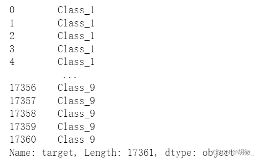
y_resampled

from sklearn.preprocessing import LabelEncoderle = LabelEncoder()
y_resampled = le.fit_transform(y_resampled)
y_resampled

（4）分割数据

from sklearn.model_selection import train_test_splitx_train,x_test,y_train,y_test = train_test_split(x_resampled,y_resampled,test_size=0.2)

4.3 模型训练

from sklearn.ensemble import RandomForestClassifierestimator = RandomForestClassifier(oob_score=True)
estimator.fit(x_train,y_train)

4.4 模型评估

本题要求使用logloss进行模型评估

y_pre = estimator.predict(x_test)
y_test,y_pre

需要注意的是：logloss在使用过程中，必须要求将输出用one-hot表示

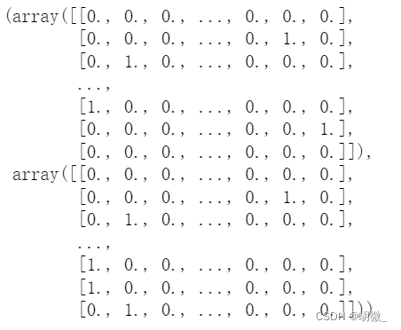
from sklearn.preprocessing import OneHotEncoderone_hot = OneHotEncoder(sparse=False)
y_pre = one_hot.fit_transform(y_pre.reshape(-1,1))
y_test = one_hot.fit_transform(y_test.reshape(-1,1))
y_test,y_pre

from sklearn.metrics import log_losslog_loss(y_test,y_pre,eps=1e-15,normalize=True)
# 7.637713870225003

改变预测值的输出模式，让输出结果为可能性的百分占比，降低logloss值

y_pre_proba = estimator.predict_proba(x_test)
y_pre_proba

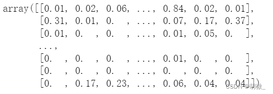
log_loss(y_test,y_pre_proba,eps=1e-15,normalize=True)
# 0.7611795612521034

由此可见，log_loss值下降了许多

4.5 模型调优

（1）确定最优的n_estimators

# 确定n_estimators的取值范围
tuned_parameters = range(10,200,10)# 创建添加accuracy的一个numpy
accuracy_t = np.zeros(len(tuned_parameters)) # 创建添加error的一个numpy
error_t = np.zeros(len(tuned_parameters)) # 调优过程实现
for i,one_parameter in enumerate(tuned_parameters):estimator = RandomForestClassifier(n_estimators=one_parameter,max_depth=10,max_features=10,min_samples_leaf=10,oob_score=True,random_state=0,n_jobs=-1)estimator.fit(x_train,y_train)# 输出accuracyaccuracy_t[i] = estimator.oob_score_# 输出log_lossy_pre = estimator.predict_proba(x_test)error_t[i] = log_loss(y_test,y_pre,eps=1e-15,normalize=True)# 优化结果过程可视化 
fig,axes = plt.subplots(nrows=1,ncols=2,figsize=(20,4),dpi=100)
axes[0].plot(tuned_parameters,accuracy_t)
axes[1].plot(tuned_parameters,error_t)axes[0].set_xlabel("n_estimators")
axes[0].set_ylabel("accuracy_t")axes[1].set_xlabel("n_estimators")
axes[1].set_ylabel("error_t")axes[0].grid()
axes[1].grid()

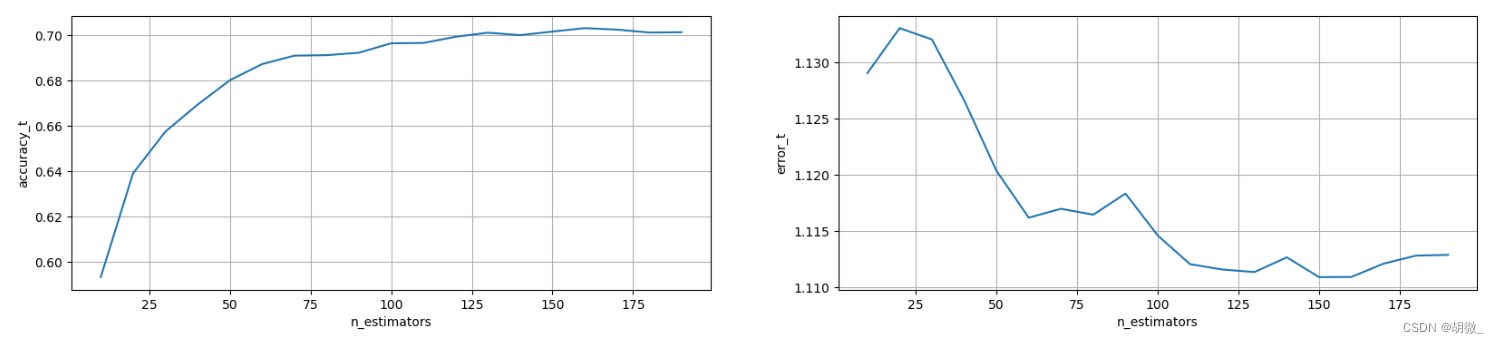
经过图像展示，最后确定n_estimators=175时，效果不错

（2）确定最优的max_depth

# 确定max_depth的取值范围
tuned_parameters = range(10,100,10)# 创建添加accuracy的一个numpy
accuracy_t = np.zeros(len(tuned_parameters)) # 创建添加error的一个numpy
error_t = np.zeros(len(tuned_parameters)) # 调优过程实现
for i,one_parameter in enumerate(tuned_parameters):estimator = RandomForestClassifier(n_estimators=175,max_depth=one_parameter,max_features=10,min_samples_leaf=10,oob_score=True,random_state=0,n_jobs=-1)estimator.fit(x_train,y_train)# 输出accuracyaccuracy_t[i] = estimator.oob_score_# 输出log_lossy_pre = estimator.predict_proba(x_test)error_t[i] = log_loss(y_test,y_pre,eps=1e-15,normalize=True)# 优化结果过程可视化 
fig,axes = plt.subplots(nrows=1,ncols=2,figsize=(20,4),dpi=100)
axes[0].plot(tuned_parameters,accuracy_t)
axes[1].plot(tuned_parameters,error_t)axes[0].set_xlabel("max_depth")
axes[0].set_ylabel("accuracy_t")axes[1].set_xlabel("max_depth")
axes[1].set_ylabel("error_t")axes[0].grid()
axes[1].grid()

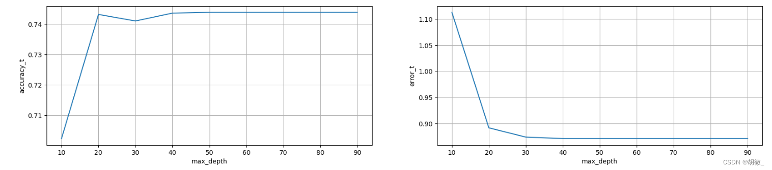
经过图像展示，最后确定max_depth=30时，效果不错

（3）确定最优的max_features

# 确定max_features取值范围
tuned_parameters = range(5,40,5)# 创建添加accuracy的一个numpy
accuracy_t = np.zeros(len(tuned_parameters)) # 创建添加error的一个numpy
error_t = np.zeros(len(tuned_parameters)) # 调优过程实现
for i,one_parameter in enumerate(tuned_parameters):estimator = RandomForestClassifier(n_estimators=175,max_depth=30,max_features=one_parameter,min_samples_leaf=10,oob_score=True,random_state=0,n_jobs=-1)estimator.fit(x_train,y_train)# 输出accuracyaccuracy_t[i] = estimator.oob_score_# 输出log_lossy_pre = estimator.predict_proba(x_test)error_t[i] = log_loss(y_test,y_pre,eps=1e-15,normalize=True)# 优化结果过程可视化
fig,axes = plt.subplots(nrows=1,ncols=2,figsize=(20,4),dpi=100)
axes[0].plot(tuned_parameters,accuracy_t)
axes[1].plot(tuned_parameters,error_t)axes[0].set_xlabel("max_features")
axes[0].set_ylabel("accuracy_t")axes[1].set_xlabel("max_features")
axes[1].set_ylabel("error_t")axes[0].grid()
axes[1].grid()

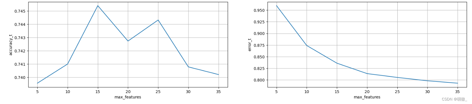
经过图像展示，最后确定max_features=15时，效果不错

（4）确定最优的min_samples_leaf

# 确定n_estimators的取值范围
tuned_parameters = range(1,10,2)# 创建添加accuracy的一个numpy
accuracy_t = np.zeros(len(tuned_parameters)) # 创建添加error的一个numpy
error_t = np.zeros(len(tuned_parameters)) # 调优过程实现
for i,one_parameter in enumerate(tuned_parameters):estimator = RandomForestClassifier(n_estimators=175,max_depth=30,max_features=15,min_samples_leaf=one_parameter,oob_score=True,random_state=0,n_jobs=-1)estimator.fit(x_train,y_train)# 输出accuracyaccuracy_t[i] = estimator.oob_score_# 输出log_lossy_pre = estimator.predict_proba(x_test)error_t[i] = log_loss(y_test,y_pre,eps=1e-15,normalize=True)# 优化结果过程可视化
fig,axes = plt.subplots(nrows=1,ncols=2,figsize=(20,4),dpi=100)
axes[0].plot(tuned_parameters,accuracy_t)
axes[1].plot(tuned_parameters,error_t)axes[0].set_xlabel("min_samples_leaf")
axes[0].set_ylabel("accuracy_t")axes[1].set_xlabel("min_samples_leaf")
axes[1].set_ylabel("error_t")axes[0].grid()
axes[1].grid()

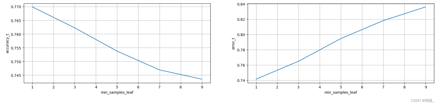
经过图像展示，最后确定min_samples_leaf=1时，效果不错

（5）确定最优模型

estimator = RandomForestClassifier(n_estimators=175,max_depth=30,max_features=15,min_samples_leaf=1,oob_score=True,random_state=0,n_jobs=-1)
estimator.fit(x_train,y_train)
y_pre_proba = estimator.predict_proba(x_test)
log_loss(y_test,y_pre_proba)
# 0.7413651159154644

4.6 生成提交数据

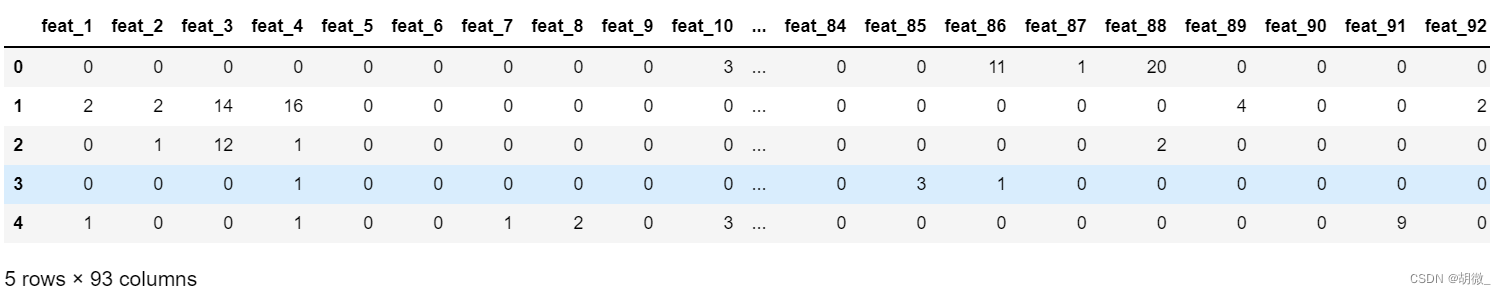
test_data = pd.read_csv("./Data/otto/test.csv")
test_data.head()

注意：测试集是没有目标值的

为了便于模型预测，删去 id 列，仅保留特征列

test_data_drop_id = test_data.drop("id",axis=1)
test_data_drop_id.head()

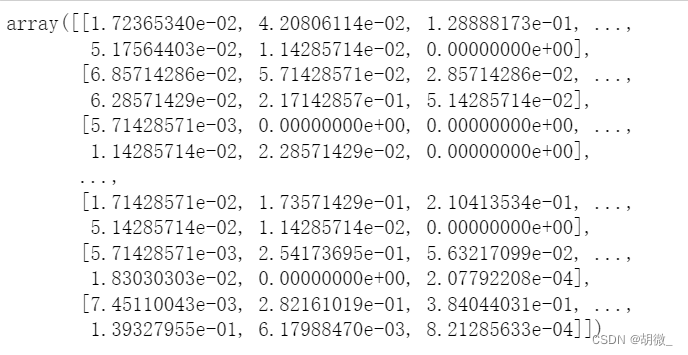
y_pre_test = estimator.predict_proba(test_data_drop_id)
y_pre_test

按要求生成列名

result_data = pd.DataFrame(y_pre_test,columns=["Class_"+str(i) for i in range(1,10)])
result_data.head()

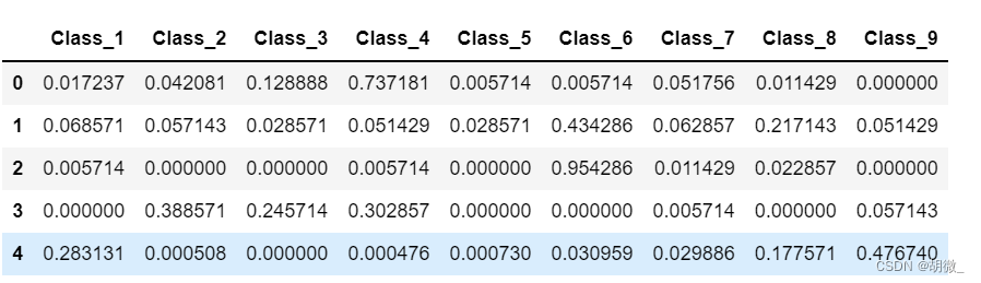
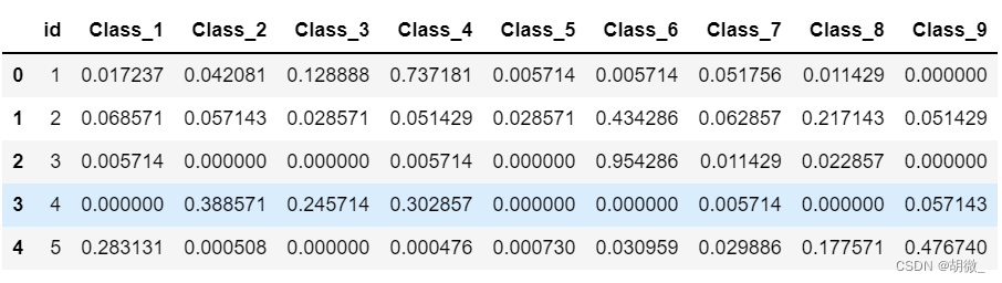
在第一列添加 id 列

result_data.insert(loc=0,column="id",value=test_data.id)
result_data.head()

生成提交数据的csv文件

result_data.to_csv("./Data/otto/Submission.csv",index=False)