本文主要是介绍MATLAB算法实战应用案例精讲-【优化算法】树木生长算法(TGA)(附MATLAB代码实现),希望对大家解决编程问题提供一定的参考价值,需要的开发者们随着小编来一起学习吧!
前言
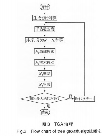
Armin Cheraghalipour 根据树木生长的特点于2017 年提出了一种新的元启发式优化算法TGA该算将始定量的群按照解的适应度从高到低排序,分成4组具有不同功能的种群。每次迭代分别进行处理。
算法原理
算法流程图
代码实现
MATLAB
TGA.m
% "Tree growth algorithm (TGA): A novel approach for solving
% optimization problems"
function [fitG,Xgb,curve] = TGA(N, max_Iter, lb,ub ,dim, fun)
% Parameters
num_tree1  = 3;    % size of first group
num_tree2  = 5;    % size of second group
num_tree4  = 3;    % size of fourth group
theta      = 0.8;  % tree reduction rate of power
lambda     = 0.5;  % control nearest tree
% Limit number of N4 to N1
if num_tree4 > num_tree1 + num_tree2num_tree4 = num_tree1 + num_tree2;
end
% Initial
X   = zeros(N,dim);
for i = 1:Nfor d = 1:dimX(i,d) = lb + (ub - lb) * rand();end
end
% Fitness
fit  = zeros(1,N);
fitG = inf;
for i = 1:Nfit(i) = fun(X(i,:));% Best if fit(i) < fitGfitG = fit(i); Xgb  = X(i,:);end
end
% Sort tree from best to worst
[fit, idx] = sort(fit,'ascend');
X          = X(idx,:);
% Initial
dist = zeros(1,num_tree1 + num_tree2);
X1   = zeros(num_tree1,dim);
Xnew = zeros(num_tree4,dim);
Fnew = zeros(1,num_tree4);
curve = zeros(1,max_Iter);
curve(1) = fitG;
t = 2;
% Iterations
while t <= max_Iter% {1} Best trees groupfor i = 1:num_tree1r1 = rand();for d = 1:dim% Local search (1)X1(i,d) = (X(i,d) / theta) + r1 * X(i,d);end% BoundaryXB = X1(i,:); XB(XB > ub) = ub; XB(XB < lb) = lb;X1(i,:) = XB;% FitnessfitT = fun(X1(i,:));% Greedy selectionif fitT <= fit(i)X(i,:) = X1(i,:);fit(i) = fitT;endend% {2} Competitive for light tree groupX_ori = X;for i = num_tree1 + 1 : num_tree1 + num_tree2% Neighbor treefor j = 1 : num_tree1 + num_tree2           if j ~= i% Compute Euclidean distance (2)dist(j) = sqrt(sum((X_ori(j,:) - X_ori(i,:)) .^ 2));else% Solve same tree problemdist(j) = inf;endend% Find 2 trees with shorter distance[~, idx] = sort(dist,'ascend'); T1       = X_ori(idx(1),:);T2       = X_ori(idx(2),:); % Alpha in [0,1]alpha    = rand();for d = 1:dim% Compute linear combination between 2 shorter tree (3)y = lambda * T1(d) + (1 - lambda) * T2(d);% Move tree i between 2 adjacent trees (4)X(i,d) = X(i,d) + alpha * y;end% BoundaryXB = X(i,:); XB(XB > ub) = ub; XB(XB < lb) = lb;X(i,:) = XB;% Fitnessfit(i) = fun(X(i,:));end% {3} Remove and replace groupfor i = num_tree1 + num_tree2 + 1 : Nfor d = 1:dim% Generate new tree by remove worst treeX(i,d) = lb + (ub - lb) * rand();end% Fitnessfit(i) = fun(X(i,:) );end% {4} Reproduction groupfor i = 1:num_tree4% Random a best treer     = randi([1,num_tree1]);Xbest = X(r,:);% Mask operatormask  = randi([0,1],1,dim);% Mask opration between new & best treesfor d = 1:dim% Generate new solution Xn = lb + (ub - lb) * rand();if mask(d) == 1Xnew(i,d) = Xbest(d);elseif mask(d) == 0% Generate new treeXnew(i,d) = Xn;endend% FitnessFnew(i) = fun(Xnew(i,:));end% Sort population get best nPop treesXX        = [X; Xnew];FF        = [fit, Fnew];[FF, idx] = sort(FF,'ascend');X         = XX(idx(1:N),:);fit       = FF(1:N);% Global bestif fit(1) < fitGfitG = fit(1); Xgb  = X(1,:);endcurve(t) = fitG;t = t + 1;
end
end
func_plot.m
% This function draw the benchmark functionsfunction func_plot(func_name)[lb,ub,dim,fobj]=Get_Functions_details(func_name);switch func_name case 'F1' x=-100:2:100; y=x; %[-100,100]case 'F2' x=-100:2:100; y=x; %[-10,10]case 'F3' x=-100:2:100; y=x; %[-100,100]case 'F4' x=-100:2:100; y=x; %[-100,100]case 'F5' x=-200:2:200; y=x; %[-5,5]case 'F6' x=-100:2:100; y=x; %[-100,100]case 'F7' x=-1:0.03:1;  y=x;  %[-1,1]case 'F8' x=-500:10:500;y=x; %[-500,500]case 'F9' x=-5:0.1:5;   y=x; %[-5,5]    case 'F10' x=-20:0.5:20; y=x;%[-500,500]case 'F11' x=-500:10:500; y=x;%[-0.5,0.5]case 'F12' x=-10:0.1:10; y=x;%[-pi,pi]case 'F13' x=-5:0.08:5; y=x;%[-3,1]case 'F14' x=-100:2:100; y=x;%[-100,100]case 'F15' x=-5:0.1:5; y=x;%[-5,5]case 'F16' x=-1:0.01:1; y=x;%[-5,5]case 'F17' x=-5:0.1:5; y=x;%[-5,5]case 'F18' x=-5:0.06:5; y=x;%[-5,5]case 'F19' x=-5:0.1:5; y=x;%[-5,5]case 'F20' x=-5:0.1:5; y=x;%[-5,5]        case 'F21' x=-5:0.1:5; y=x;%[-5,5]case 'F22' x=-5:0.1:5; y=x;%[-5,5]     case 'F23' x=-5:0.1:5; y=x;%[-5,5]
end    L=length(x);
f=[];for i=1:Lfor j=1:Lif strcmp(func_name,'F15')==0 && strcmp(func_name,'F19')==0 && strcmp(func_name,'F20')==0 && strcmp(func_name,'F21')==0 && strcmp(func_name,'F22')==0 && strcmp(func_name,'F23')==0f(i,j)=fobj([x(i),y(j)]);endif strcmp(func_name,'F15')==1f(i,j)=fobj([x(i),y(j),0,0]);endif strcmp(func_name,'F19')==1f(i,j)=fobj([x(i),y(j),0]);endif strcmp(func_name,'F20')==1f(i,j)=fobj([x(i),y(j),0,0,0,0]);end       if strcmp(func_name,'F21')==1 || strcmp(func_name,'F22')==1 ||strcmp(func_name,'F23')==1f(i,j)=fobj([x(i),y(j),0,0]);end          end
endsurfc(x,y,f,'LineStyle','none');end
Get_Functions_details.m
% This function containts full information and implementations of the benchmark
% functions in Table 1, Table 2, and Table 3 in the paper% lb is the lower bound: lb=[lb_1,lb_2,...,lb_d]
% up is the uppper bound: ub=[ub_1,ub_2,...,ub_d]
% dim is the number of variables (dimension of the problem)function [lb,ub,dim,fobj] = Get_Functions_details(F)switch Fcase 'F1'fobj = @F1;lb=-100;ub=100;dim=30;case 'F2'fobj = @F2;lb=-10;ub=10;dim=30;case 'F3'fobj = @F3;lb=-100;ub=100;dim=30;case 'F4'fobj = @F4;lb=-100;ub=100;dim=30;case 'F5'fobj = @F5;lb=-30;ub=30;dim=30;case 'F6'fobj = @F6;lb=-100;ub=100;dim=30;case 'F7'fobj = @F7;lb=-1.28;ub=1.28;dim=30;case 'F8'fobj = @F8;lb=-500;ub=500;dim=30;case 'F9'fobj = @F9;lb=-5.12;ub=5.12;dim=30;case 'F10'fobj = @F10;lb=-32;ub=32;dim=30;case 'F11'fobj = @F11;lb=-600;ub=600;dim=30;case 'F12'fobj = @F12;lb=-50;ub=50;dim=30;case 'F13'fobj = @F13;lb=-50;ub=50;dim=30;case 'F14'fobj = @F14;lb=-65.536;ub=65.536;dim=2;case 'F15'fobj = @F15;lb=-5;ub=5;dim=4;case 'F16'fobj = @F16;lb=-5;ub=5;dim=2;case 'F17'fobj = @F17;lb=[-5,0];ub=[10,15];dim=2;case 'F18'fobj = @F18;lb=-2;ub=2;dim=2;case 'F19'fobj = @F19;lb=0;ub=1;dim=3;case 'F20'fobj = @F20;lb=0;ub=1;dim=6;     case 'F21'fobj = @F21;lb=0;ub=10;dim=4;    case 'F22'fobj = @F22;lb=0;ub=10;dim=4;    case 'F23'fobj = @F23;lb=0;ub=10;dim=4;
endend% F1function o = F1(x)
o=sum(x.^2);
end% F2function o = F2(x)
o=sum(abs(x))+prod(abs(x));
end% F3function o = F3(x)
dim=size(x,2);
o=0;
for i=1:dimo=o+sum(x(1:i))^2;
end
end% F4function o = F4(x)
o=max(abs(x));
end% F5function o = F5(x)
dim=size(x,2);
o=sum(100*(x(2:dim)-(x(1:dim-1).^2)).^2+(x(1:dim-1)-1).^2);
end% F6function o = F6(x)
o=sum(abs((x+.5)).^2);
end% F7function o = F7(x)
dim=size(x,2);
o=sum([1:dim].*(x.^4))+rand;
end% F8function o = F8(x)
o=sum(-x.*sin(sqrt(abs(x))));
end% F9function o = F9(x)
dim=size(x,2);
o=sum(x.^2-10*cos(2*pi.*x))+10*dim;
end% F10function o = F10(x)
dim=size(x,2);
o=-20*exp(-.2*sqrt(sum(x.^2)/dim))-exp(sum(cos(2*pi.*x))/dim)+20+exp(1);
end% F11function o = F11(x)
dim=size(x,2);
o=sum(x.^2)/4000-prod(cos(x./sqrt([1:dim])))+1;
end% F12function o = F12(x)
dim=size(x,2);
o=(pi/dim)*(10*((sin(pi*(1+(x(1)+1)/4)))^2)+sum((((x(1:dim-1)+1)./4).^2).*...
(1+10.*((sin(pi.*(1+(x(2:dim)+1)./4)))).^2))+((x(dim)+1)/4)^2)+sum(Ufun(x,10,100,4));
end% F13function o = F13(x)
dim=size(x,2);
o=.1*((sin(3*pi*x(1)))^2+sum((x(1:dim-1)-1).^2.*(1+(sin(3.*pi.*x(2:dim))).^2))+...
((x(dim)-1)^2)*(1+(sin(2*pi*x(dim)))^2))+sum(Ufun(x,5,100,4));
end% F14function o = F14(x)
aS=[-32 -16 0 16 32 -32 -16 0 16 32 -32 -16 0 16 32 -32 -16 0 16 32 -32 -16 0 16 32;,...
-32 -32 -32 -32 -32 -16 -16 -16 -16 -16 0 0 0 0 0 16 16 16 16 16 32 32 32 32 32];for j=1:25bS(j)=sum((x'-aS(:,j)).^6);
end
o=(1/500+sum(1./([1:25]+bS))).^(-1);
end% F15function o = F15(x)
aK=[.1957 .1947 .1735 .16 .0844 .0627 .0456 .0342 .0323 .0235 .0246];
bK=[.25 .5 1 2 4 6 8 10 12 14 16];bK=1./bK;
o=sum((aK-((x(1).*(bK.^2+x(2).*bK))./(bK.^2+x(3).*bK+x(4)))).^2);
end% F16function o = F16(x)
o=4*(x(1)^2)-2.1*(x(1)^4)+(x(1)^6)/3+x(1)*x(2)-4*(x(2)^2)+4*(x(2)^4);
end% F17function o = F17(x)
o=(x(2)-(x(1)^2)*5.1/(4*(pi^2))+5/pi*x(1)-6)^2+10*(1-1/(8*pi))*cos(x(1))+10;
end% F18function o = F18(x)
o=(1+(x(1)+x(2)+1)^2*(19-14*x(1)+3*(x(1)^2)-14*x(2)+6*x(1)*x(2)+3*x(2)^2))*...(30+(2*x(1)-3*x(2))^2*(18-32*x(1)+12*(x(1)^2)+48*x(2)-36*x(1)*x(2)+27*(x(2)^2)));
end% F19function o = F19(x)
aH=[3 10 30;.1 10 35;3 10 30;.1 10 35];cH=[1 1.2 3 3.2];
pH=[.3689 .117 .2673;.4699 .4387 .747;.1091 .8732 .5547;.03815 .5743 .8828];
o=0;
for i=1:4o=o-cH(i)*exp(-(sum(aH(i,:).*((x-pH(i,:)).^2))));
end
end% F20function o = F20(x)
aH=[10 3 17 3.5 1.7 8;.05 10 17 .1 8 14;3 3.5 1.7 10 17 8;17 8 .05 10 .1 14];
cH=[1 1.2 3 3.2];
pH=[.1312 .1696 .5569 .0124 .8283 .5886;.2329 .4135 .8307 .3736 .1004 .9991;...
.2348 .1415 .3522 .2883 .3047 .6650;.4047 .8828 .8732 .5743 .1091 .0381];
o=0;
for i=1:4o=o-cH(i)*exp(-(sum(aH(i,:).*((x-pH(i,:)).^2))));
end
end% F21function o = F21(x)
aSH=[4 4 4 4;1 1 1 1;8 8 8 8;6 6 6 6;3 7 3 7;2 9 2 9;5 5 3 3;8 1 8 1;6 2 6 2;7 3.6 7 3.6];
cSH=[.1 .2 .2 .4 .4 .6 .3 .7 .5 .5];o=0;
for i=1:5o=o-((x-aSH(i,:))*(x-aSH(i,:))'+cSH(i))^(-1);
end
end% F22function o = F22(x)
aSH=[4 4 4 4;1 1 1 1;8 8 8 8;6 6 6 6;3 7 3 7;2 9 2 9;5 5 3 3;8 1 8 1;6 2 6 2;7 3.6 7 3.6];
cSH=[.1 .2 .2 .4 .4 .6 .3 .7 .5 .5];o=0;
for i=1:7o=o-((x-aSH(i,:))*(x-aSH(i,:))'+cSH(i))^(-1);
end
end% F23function o = F23(x)
aSH=[4 4 4 4;1 1 1 1;8 8 8 8;6 6 6 6;3 7 3 7;2 9 2 9;5 5 3 3;8 1 8 1;6 2 6 2;7 3.6 7 3.6];
cSH=[.1 .2 .2 .4 .4 .6 .3 .7 .5 .5];o=0;
for i=1:10o=o-((x-aSH(i,:))*(x-aSH(i,:))'+cSH(i))^(-1);
end
endfunction o=Ufun(x,a,k,m)
o=k.*((x-a).^m).*(x>a)+k.*((-x-a).^m).*(x<(-a));
end
main.m
%_________________________________________________________________________________
%_________________________________________________________________________________
clear all
clcSearchAgents_no=30; % Number of search agents
Function_name='F1'; % Name of the test function that can be from F1 to F23
Max_iteration=500; % Maximum numbef of iterations
% Load details of the selected benchmark function
[lb,ub,dim,fobj]=Get_Functions_details(Function_name);
[Best_score,Best_pos,cg_curve]=TGA(SearchAgents_no,Max_iteration,lb,ub,dim,fobj);display(['The best solution obtained by OPTIMIZER is : ', num2str(Best_pos)]);
display(['The best optimal value of the objective function found by OPTIMIZER is : ', num2str(Best_score)]);%Draw objective space
figure,
subplot(1,2,1);
func_plot(Function_name);
title([Function_name])
xlabel('x_1');
ylabel('x_2');
zlabel([Function_name,'( x_1 , x_2 )'])
set(gca,'color','none')
grid offsubplot(1,2,2);
semilogy(cg_curve,'Color','b','LineWidth',4);
title('Convergence curve')
xlabel('Iteration');
ylabel('Best fitness obtained so far');
axis tight
grid off
box on
legend('TGA')
这篇关于MATLAB算法实战应用案例精讲-【优化算法】树木生长算法(TGA)(附MATLAB代码实现)的文章就介绍到这儿,希望我们推荐的文章对编程师们有所帮助!


