【立体匹配和深度估计 2】Middlebury Stereo Datasets

参考《高精度立体匹配算法研究》

vision.middlebury.edu 由 Daniel Scharstein 和 Richard Szeliski 及其他研究人员维护。Middlebury Stereo Vision Page 主要提供立体匹配算法的在线评价和数据下载服务。它由《A taxonomy and evaluation of dense two-frame stereo correspondence algorithms》这篇文章发展而来。
这篇文章主要介绍其数据集 Middlebury Stereo Datasets。

文章目录
1. Middlebury Stereo Datasets
1.1 2001 Stereo datasets with ground truth
1.2 2003 Stereo datasets with ground truth
1.3 2005 Stereo datasets with ground truth
1.4 2006 Stereo datasets with ground truth
1.5 2014 Stereo datasets with ground truth
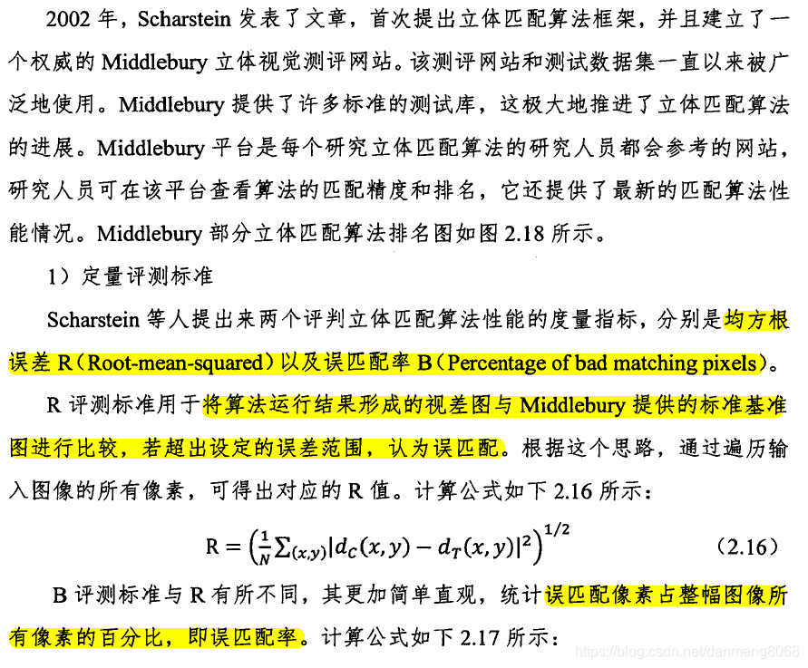
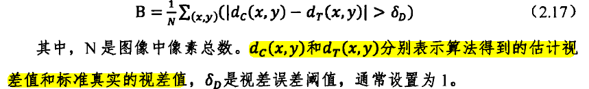
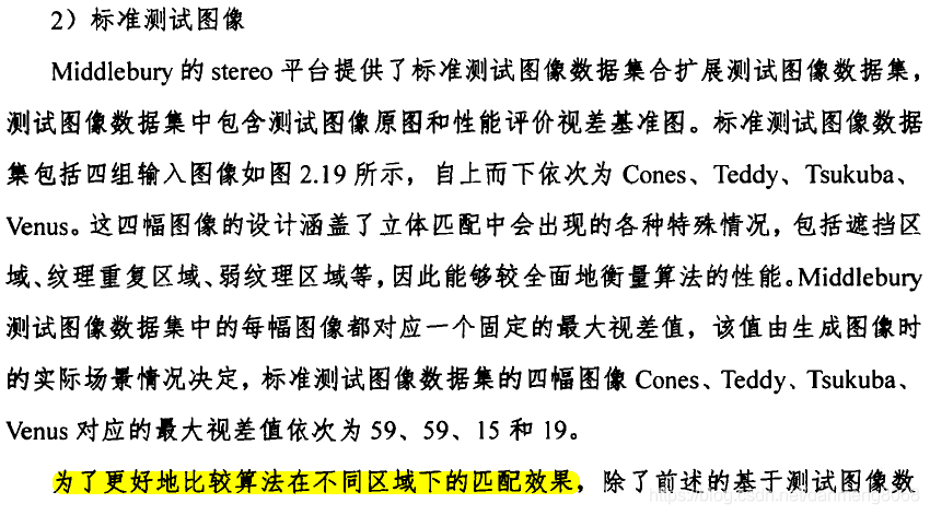
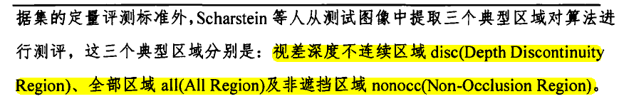
2. Middlebury Stereo Evaluation
1. Middlebury Stereo Datasets
1.1 2001 Stereo datasets with ground truth
2001 Stereo datasets 由 Daniel Scharstein, Padma Ugbabe, and Rick Szeliski创建。每套子集包含9张图像(im0.ppm - im8.ppm) 和对应 images 2 和 6 的实际真值视差图(disp2.pgm anddisp6.pgm)。也就是说，9张图像是沿水平线的序列，其中 im2.ppm 为左视图，im6.ppm 为右视图，disp2.pgm为左视差图，disp6.pgm为右视差图。

每个实际真值视差图中每个点的视差值被放大了8倍。举例说明，在disp2.pgm中某点的值为100，意味着im2.ppm(左图)中的该位置的像素点和与之对应的im6.ppm(右图)中的像素点的水平像素距离为12.5。

1.2 2003 Stereo datasets with ground truth
2003 Stereo datasets 由Daniel Scharstein, Alexander Vandenberg-Rodes, 和 Rick Szeliski 创建。它包含高分辨率的双目图像序列，以及精确到像素水平的实际真值视差图。实际真值视差图由结构光这种新技术采集获得，因而不需要矫正光照映射。

数据描述:

Quarter-size (450 x 375) versions of our new data sets “Cones” and “Teddy” are available for download below. Each data set contains 9 color images (im0…im8) and 2 disparity maps (disp2 and disp6). The 9 color images form a multi-baseline stereo sequence, i.e., they are taken from equally-spaced viewpoints along the x-axis from left to right. The images are rectified so that all image motion is purely horizontal. To test a two-view stereo algorithm, the two reference views im2 (left) and im6 (right) should be used. Ground-truth disparites with quarter-pixel accuracy are provided for these two views. Disparities are encoded using a scale factor 4 for gray levels 1 … 255, while gray level 0 means “unknown disparity”. Therefore, the encoded disparity range is 0.25 … 63.75 pixels.

F - full size: 1800 x 1500
H - half size: 900 x 750
Q - quarter size: 450 x 375 (same as above)

1.3 2005 Stereo datasets with ground truth
These 9 datasets of 2005 Stereo datasets were created by Anna Blasiak, Jeff Wehrwein, and Daniel Scharstein at Middlebury College in the summer of 2005, and were published in conjunction with two CVPR 2007 papers [3, 4]. Each image below links to a directory containing the full-size views and disparity maps. Shown are the left views; moving the mouse over the images shows the right views. We’re withholding the true disparity maps for three of the sequences (Computer, Drumsticks, and Dwarves) which we may use in future evaluations.

Dataset description:

Each dataset consists of 7 views (0…6) taken under three different illuminations (1…3) and with three different exposures (0…2). Here’s an overview. Disparity maps are provided for views 1 and 5. The images are rectified and radial distortion has been removed. We provide each dataset in three resolutions: full-size (width: 1330…1390, height: 1110), half-size (width: 665…695, height: 555), and third-size (width: 443…463, height: 370). The files are organized as follows:

{Full,Half,Third}Size/
  SCENE/
    disp1.png
    disp5.png
    dmin.txt
    Illum{1,2,3}/
      Exp{0,1,2}/
        exposure_ms.txt
        view{0-6}.png

The file “exposure_ms.txt” lists the exposure time in milliseconds. The disparity images relate views 1 and 5. For the full-size images, disparities are represented “as is”, i.e., intensity 60 means the disparity is 60. The exception is intensity 0, which means unknown disparity. In the half-size and third-size versions, the intensity values of the disparity maps need to be divided by 2 and 3, respectively. To map the disparities into 3D coordinates, add the value in “dmin.txt” to each disparity value, since the images and disparity maps were cropped. The focal length is 3740 pixels, and the baseline is 160mm. We do not provide any other calibration data. Occlusion maps can be generated by crosschecking the pair of disparity maps.

1.4 2006 Stereo datasets with ground truth
These 21 datasets of 2006 Stereo datasets were created by Brad Hiebert-Treuer, Sarri Al Nashashibi, and Daniel Scharstein at Middlebury College in the summer of 2006, and were published in conjunction with two CVPR 2007 papers [3, 4]. Each image below links to a directory containing the full-size views and disparity maps. Shown are the left views; moving the mouse over the images shows the right views.

Dataset description:

Each dataset consists of 7 views (0…6) taken under three different illuminations (1…3) and with three different exposures (0…2). Here’s an overview. Disparity maps are provided for views 1 and 5. The images are rectified and radial distortion has been removed. We provide each dataset in three resolutions: full-size (width: 1240…1396, height: 1110), half-size (width: 620…698, height: 555), and third-size (width: 413…465, height: 370). The files are organized as follows:

{Full,Half,Third}Size/
  SCENE/
    disp1.png
    disp5.png
    dmin.txt
    Illum{1,2,3}/
      Exp{0,1,2}/
        exposure_ms.txt
        view{0-6}.png

The file “exposure_ms.txt” lists the exposure time in milliseconds. The disparity images relate views 1 and 5. For the full-size images, disparities are represented “as is”, i.e., intensity 60 means the disparity is 60. The exception is intensity 0, which means unknown disparity. In the half-size and third-size versions, the intensity values of the disparity maps need to be divided by 2 and 3, respectively. To map the disparities into 3D coordinates, add the value in “dmin.txt” to each disparity value, since the images and disparity maps were cropped. The focal length is 3740 pixels, and the baseline is 160mm. We do not provide any other calibration data. Occlusion maps can be generated by crosschecking the pair of disparity maps.

1.5 2014 Stereo datasets with ground truth
These 33 datasets of 2014 Stereo datasets were created by Nera Nesic, Porter Westling, Xi Wang, York Kitajima, Greg Krathwohl, and Daniel Scharstein at Middlebury College during 2011-2013, and refined with Heiko Hirschmüller at the DLR Germany during 2014. A detailed description of the acquisition process can be found in our GCPR 2014 paper [5]. 20 of the datasets are used in the new Middlebury Stereo Evaluation (10 each for training and test sets). Except for the 10 test datasets, we provide links to directories containing the full-size views and disparity maps.

Dataset description

Each dataset consists of 2 views taken under several different illuminations and exposures. The files are organized as follows:

SCENE-{perfect,imperfect}/     -- each scene comes with perfect and imperfect calibration (see paper)
  ambient/                     -- directory of all input views under ambient lighting
    L{1,2,...}/                -- different lighting conditions
      im0e{0,1,2,...}.png      -- left view under different exposures
      im1e{0,1,2,...}.png      -- right view under different exposures
  calib.txt                    -- calibration information
  im{0,1}.png                  -- default left and right view
  im1E.png                     -- default right view under different exposure
  im1L.png                     -- default right view with different lighting
  disp{0,1}.pfm                -- left and right GT disparities
  disp{0,1}-n.png              -- left and right GT number of samples (* perfect only)
  disp{0,1}-sd.pfm             -- left and right GT sample standard deviations (* perfect only)
  disp{0,1}y.pfm               -- left and right GT y-disparities (* imperfect only)

Calibration file format
Here is a sample calib.txt file for one of the full-size training image pairs:

cam0=[3997.684 0 1176.728; 0 3997.684 1011.728; 0 0 1]
cam1=[3997.684 0 1307.839; 0 3997.684 1011.728; 0 0 1]
doffs=131.111
baseline=193.001
width=2964
height=1988
ndisp=280
isint=0
vmin=31
vmax=257
dyavg=0.918
dymax=1.516

The calibration files provided with the test image pairs used in the stereo evaluation only contain the first 7 lines, up to the “ndisp” parameter.

Explanation:

cam0,1:        camera matrices for the rectified views, in the form [f 0 cx; 0 f cy; 0 0 1], where
  f:           focal length in pixels
  cx, cy:      principal point  (note that cx differs between view 0 and 1)

doffs:         x-difference of principal points, doffs = cx1 - cx0

baseline:      camera baseline in mm

width, height: image size

ndisp:         a conservative bound on the number of disparity levels;
               the stereo algorithm MAY utilize this bound and search from d = 0 .. ndisp-1

isint:         whether the GT disparites only have integer precision (true for the older datasets;
               in this case submitted floating-point disparities are rounded to ints before evaluating)

vmin, vmax:    a tight bound on minimum and maximum disparities, used for color visualization;
               the stereo algorithm MAY NOT utilize this information

dyavg, dymax:  average and maximum absolute y-disparities, providing an indication of
               the calibration error present in the imperfect datasets.

To convert from the floating-point disparity value d [pixels] in the .pfm file to depth Z [mm] the following equation can be used:

Z = baseline * f / (d + doffs)

Note that the image viewer “sv” and mesh viewer “plyv” provided by our software cvkit can read the calib.txt files and provide this conversion automatically when viewing .pfm disparity maps as 3D meshes.

2. Middlebury Stereo Evaluation
————————————————
版权声明：本文为CSDN博主「RadiantJeral」的原创文章，遵循 CC 4.0 BY-SA 版权协议，转载请附上原文出处链接及本声明。
原文链接：https://blog.csdn.net/RadiantJeral/article/details/85172432

【立体匹配和深度估计 3】Computer Vision Toolkit (cvkit)

https://blog.csdn.net/RadiantJeral/article/details/86008558