本文主要是介绍基于机器学习和奇异值分解SVD的电池剩余使用寿命预测(Python),希望对大家解决编程问题提供一定的参考价值,需要的开发者们随着小编来一起学习吧!
采用k-最近邻KNN和随机森林算法建立预测模型。
import pandas as pd
from sklearn.model_selection import train_test_split
from sklearn.svm import SVC  # Support Vector Classifier
from sklearn.preprocessing import StandardScaler
from sklearn.metrics import accuracy_score, classification_report
from sklearn.decomposition import TruncatedSVD
from ydata_profiling import ProfileReport
from sklearn.metrics import mean_squared_error
import timeimport seaborn as sns
from importlib import reload
import matplotlib.pyplot as plt
import matplotlib
import warningsfrom IPython.display import display, HTML
import plotly.graph_objects as go
import plotly.express as px
from plotly.subplots import make_subplots
import plotly.io as pio# Configure Jupyter Notebook
pd.set_option('display.max_columns', None)
pd.set_option('display.max_rows', 500)
pd.set_option('display.expand_frame_repr', False)
display(HTML("<style>div.output_scroll { height: 35em; }</style>"))
dataset = pd.read_csv('Battery_RUL.csv')profile = ProfileReport(dataset)
profileSummarize dataset: 0%| | 0/5 [00:00<?, ?it/s]Generate report structure: 0%| | 0/1 [00:00<?, ?it/s]Render HTML: 0%| | 0/1 [00:00<?, ?it/s]y = dataset['RUL']x = dataset.drop(columns=['RUL'])X_train, X_test, y_train, y_test = train_test_split(x, y, test_size=0.2, random_state=42)Singular Value Decomposition
# Step 5: Initialize and fit TruncatedSVD to your training data
n_components = 6  # Adjust the number of components based on your desired dimensionality
svd = TruncatedSVD(n_components=n_components, random_state=42)
X_train_svd = svd.fit_transform(X_train)# Step 6: Transform the test data using the fitted SVD
X_test_svd = svd.transform(X_test)
K-Nearest-Neighbors
from sklearn.neighbors import KNeighborsRegressor
start = time.time()
model = KNeighborsRegressor(n_neighbors=3).fit(X_train_svd,y_train)
end_train = time.time()
y_predictions = model.predict(X_test_svd) # These are the predictions from the test data.
end_predict = time.time()kNN = [model.score(X_test_svd,y_test), mean_squared_error(y_test,y_predictions,squared=False),end_train-start,end_predict-end_train,end_predict-start]print('R-squared error: '+ "{:.2%}".format(model.score(X_test_svd,y_test)))
print('Root Mean Squared Error: '+ "{:.2f}".format(mean_squared_error(y_test,y_predictions,squared=False)))
R-squared error: 98.93%
Root Mean Squared Error: 33.30plt.style.use('seaborn-white')
plt.rcParams['figure.figsize']=5,5 fig,ax = plt.subplots()
plt.title('Actual vs Predicted')
plt.xlabel('Actual')
plt.ylabel('Predicted')
g = sns.scatterplot(x=y_test,y=y_predictions,s=20,alpha=0.6,linewidth=1,edgecolor='black',ax=ax)
f = sns.lineplot(x=[min(y_test),max(y_test)],y=[min(y_test),max(y_test)],linewidth=4,color='gray',ax=ax)plt.annotate(text=('R-squared error: '+ "{:.2%}".format(model.score(X_test_svd,y_test)) +'\n' +'Root Mean Squared Error: '+ "{:.2f}".format(mean_squared_error(y_test,y_predictions,squared=False))),xy=(0,800),size='medium')xlabels = ['{:,.0f}'.format(x) for x in g.get_xticks()]
g.set_xticklabels(xlabels)
ylabels = ['{:,.0f}'.format(x) for x in g.get_yticks()]
g.set_yticklabels(ylabels)
sns.despine()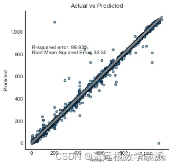
Random Forest
%%time
from sklearn.ensemble import RandomForestRegressor
start = time.time()
model = RandomForestRegressor(n_jobs=-1,n_estimators=100,min_samples_leaf=1,max_features='sqrt',# min_samples_split=2,bootstrap = True,criterion='mse',).fit(X_train_svd,y_train)
end_train = time.time()
y_predictions = model.predict(X_test_svd) # These are the predictions from the test data.
end_predict = time.time()Random_Forest = [model.score(X_test_svd,y_test), mean_squared_error(y_test,y_predictions,squared=False),end_train-start,end_predict-end_train,end_predict-start]print('R-squared error: '+ "{:.2%}".format(model.score(X_test_svd,y_test)))
print('Root Mean Squared Error: '+ "{:.2f}".format(mean_squared_error(y_test,y_predictions,squared=False)))
R-squared error: 99.75%
Root Mean Squared Error: 15.97
CPU times: total: 3.34 s
Wall time: 389 msplt.style.use('seaborn-white')
plt.rcParams['figure.figsize']=5,5 fig,ax = plt.subplots()
plt.title('Actual vs Predicted')
plt.xlabel('Actual')
plt.ylabel('Predicted')
g = sns.scatterplot(x=y_test,y=y_predictions,s=20,alpha=0.6,linewidth=1,edgecolor='black',ax=ax)
f = sns.lineplot(x=[min(y_test),max(y_test)],y=[min(y_test),max(y_test)],linewidth=4,color='gray',ax=ax)plt.annotate(text=('R-squared error: '+ "{:.2%}".format(model.score(X_test_svd,y_test)) +'\n' +'Root Mean Squared Error: '+ "{:.2f}".format(mean_squared_error(y_test,y_predictions,squared=False))),xy=(0,800),size='medium')xlabels = ['{:,.0f}'.format(x) for x in g.get_xticks()]
g.set_xticklabels(xlabels)
ylabels = ['{:,.0f}'.format(x) for x in g.get_yticks()]
g.set_yticklabels(ylabels)
sns.despine()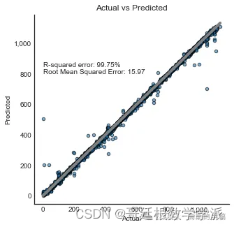
工学博士,担任《Mechanical System and Signal Processing》《中国电机工程学报》《控制与决策》等期刊审稿专家,擅长领域:现代信号处理,机器学习,深度学习,数字孪生,时间序列分析,设备缺陷检测、设备异常检测、设备智能故障诊断与健康管理PHM等。
这篇关于基于机器学习和奇异值分解SVD的电池剩余使用寿命预测(Python)的文章就介绍到这儿,希望我们推荐的文章对编程师们有所帮助!


