图像分析之图像特征点及匹配

本文主要是介绍图像分析之图像特征点及匹配，希望对大家解决编程问题提供一定的参考价值，需要的开发者们随着小编来一起学习吧！

Overview

持续更新:

• https://cgabc.xyz/posts/d12a5e77/
• https://cgabc.xyz/posts/42295323/

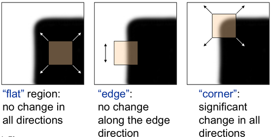
Image Corners

Types of Image Feature:

• Edges
• Corners (also known as interest points)
• Blobs (also known as regions of interest )

Harris

• cv::cornerHarris
• Harris corner detector

Define the auto-correlation surface or SSD surface or the weighted sum of squared differences:

$$\begin{array}{rl}{E}_{AC}(\Delta \mathbf{u})& =\sum _i\omega ({\mathbf{x}}_i)[{\mathbf{I}}_0({\mathbf{x}}_i+\Delta \mathbf{u})-{\mathbf{I}}_0({\mathbf{x}}_i){]}^2\\ & \approx \sum _i\omega ({\mathbf{x}}_i)[{\mathbf{I}}_0({\mathbf{x}}_i)+\nabla {\mathbf{I}}_0({\mathbf{x}}_i)\cdot \Delta \mathbf{u}-{\mathbf{I}}_0({\mathbf{x}}_i){]}^2\\ & =\sum _i\omega ({\mathbf{x}}_i)[\nabla {\mathbf{I}}_0({\mathbf{x}}_i)\cdot \Delta \mathbf{u}{]}^2\\ & =\Delta {\mathbf{u}}^T\cdot \mathbf{M}\cdot \Delta \mathbf{u}\end{array}$$

where

$$\nabla {\mathbf{I}}_0({\mathbf{x}}_i)=(\frac{\partial {\mathbf{I}}_0}{\partial x},\frac{\partial {\mathbf{I}}_0}{\partial y})({\mathbf{x}}_i)$$

written by simply the gradient

$$\nabla \mathbf{I}=[{\mathbf{I}}_x,{\mathbf{I}}_y]$$

and the auto-correlation matrix with the weighting kernel $\omega$

$$\mathbf{M}=\omega \ast \left[\begin{array}{cc}{\mathbf{I}}_x^2& {\mathbf{I}}_x{\mathbf{I}}_y\\ {\mathbf{I}}_x{\mathbf{I}}_y& {\mathbf{I}}_y^2\end{array}\right]$$

then create a score equation, which will determine if a window can contain a corner or not

$$R=det(\mathbf{M})-k(trace(\mathbf{M}){)}^2$$

where

$$det(\mathbf{M})={\lambda }_1{\lambda }_2$$

$$trace(\mathbf{M})={\lambda }_1+{\lambda }_2$$

and, ${\lambda }_1$ and ${\lambda }_2$ are the eigen values of $\mathbf{M}$, we can compute it by

$$det(\lambda E-M)=0$$

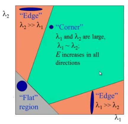
So the values of these eigen values decide whether a region is corner, edge or flat

• When $ |R| $ is small, which happens when ${\lambda }_1$ and ${\lambda }_2$ are small, the region is flat.
• When $R<0$, which happens when ${\lambda }_1>>{\lambda }_2$ or vice versa, the region is edge.
• When $R$ is large, which happens when ${\lambda }_1$ and ${\lambda }_2$ are large and ${\lambda }_1\sim {\lambda }_2$, the region is a corner.

Shi-Tomas

• cv::goodFeaturesToTrack

The Shi-Tomasi corner detector is based entirely on the Harris corner detector. However, one slight variation in a “selection criteria” made this detector much better than the original. It works quite well where even the Harris corner detector fails.

Later in 1994, J. Shi and C. Tomasi made a small modification to it in their paper Good Features to Track which shows better results compared to Harris Corner Detector.

The scoring function in Harris Corner Detector was given by (Harris corner strength):

$$\mathbf{R}={\lambda }_1{\lambda }_2-k({\lambda }_1+{\lambda }_2{)}^2$$

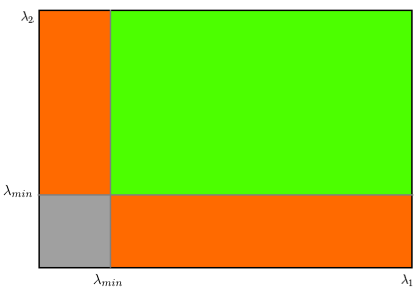
Instead of this, Shi-Tomasi proposed (get the minimum eigenvalue):

$$R=min({\lambda }_1,{\lambda }_2)$$

If $R$ is greater than a certain predefined value, it can be marked as a corner

FAST

• cv::FastFeatureDetector
• FAST Algorithm for Corner Detection

FAST (Features from Accelerated Segment Test) algorithm was proposed by Edward Rosten and Tom Drummond in their paper “Machine learning for high-speed corner detection” in 2006 (Later revised it in 2010).

Feature Detection

检测 局部像素灰度 变化明显的地方。

• 在图像中选取像素p，假设它的亮度为 $I_p$；
• 设置一个阈值 $Ｔ$；
• 以像素 $p$ 为中心，选取半径为3的 Bresenham圆 上的16个像素；
• 假设选取的圆上有连续的Ｎ个点的亮度大于 $I_p+T$ 或 $I_p-T$，则该点 $ｐ$ 可被认为是特征点（Ｎ通常取12，即为 FAST-12，其他常用的Ｎ取值有9和11，分别被成为 FAST-9 和 FAST-11）；
• 循环以上四步；

Non-maximal Suppression

FAST角点经常出现“扎堆”的情况，通过 非极大值抑制，在一定区域内仅保留响应极大值的角点，避免角点集中的问题。

SIFT

in 2004, D.Lowe, University of British Columbia, came up with a new algorithm, Scale Invariant Feature Transform (SIFT) in his paper, Distinctive Image Features from Scale-Invariant Keypoints, which extract keypoints and compute its descriptors.

该算法具有一定的仿射不变性，视角不变性，旋转不变性和光照不变性，所以在图像特征提高方面得到了最广泛的应用。

SURF

In 2006, three people, Bay, H., Tuytelaars, T. and Van Gool, L, published another paper, “SURF: Speeded Up Robust Features” which introduced a new algorithm called SURF. As name suggests, it is a speeded-up version of SIFT.

2006年，Bay和Ess等人基于SIFT算法的思路，提出了加速鲁棒特征（SURF）,该算法主要针对于SIFT算法速度太慢，计算量大的缺点，使用了近似Harr小波方法来提取特征点，这种方法就是基于Hessian行列式（DoH）的斑点特征检测方法。通过在不同的尺度上利用积分图像可以有效地计算出近似Harr小波值，简化了二阶微分模板的构建，搞高了尺度空间的特征检测的效率。

SURF算法在积分图像上使用了盒子滤波器对二阶微分模板进行了简化，从而构建了Hessian矩阵元素值，进而缩短了特征提取的时间，提高了效率。

BRIEF

• Binary Robust Independent Elementary Features

在特征点周围邻域内选取若干个像素点对，通过对这些点对的灰度值比较，将比较的结果组合成一个二进制串字符串用来描述特征点。最后，使用汉明距离来计算在特征描述子是否匹配。

BRISK

BRISK算法在特征点检测部分没有选用FAST特征点检测，而是选用了稳定性更强的AGAST算法。在特征描述子的构建中，BRISK算法通过利用简单的像素灰度值比较，进而得到一个级联的二进制比特串来描述每个特征点，这一点上原理与BRIEF是一致的。BRISK算法里采用了邻域采样模式，即以特征点为圆心，构建多个不同半径的离散化Bresenham同心圆，然后再每一个同心圆上获得具有相同间距的N个采样点。

ORB

• ORB (Oriented FAST and Rotated BRIEF)

As an OpenCV enthusiast, the most important thing about the ORB(Oriented FAST and Rotated BRIEF) is that it came from “OpenCV Labs”. This algorithm was brought up by Ethan Rublee, Vincent Rabaud, Kurt Konolige and Gary R. Bradski in their paper ORB: An efficient alternative to SIFT or SURF in 2011. As the title says, it is a good alternative to SIFT and SURF in computation cost, matching performance and mainly the patents. Yes, SIFT and SURF are patented and you are supposed to pay them for its use. But ORB is not !!!

ORB is basically a fusion of FAST keypoint detector and BRIEF descriptor with many modifications to enhance the performance.

oriented FAST

• use FAST to find keypoints, then apply Harris corner measure to find top N points among them

• multiscale

  • use pyramid to produce multiscale-features

• rotation invariance (Orientation)

  • It computes the intensity weighted centroid of the patch with located corner at center. The direction of the vector from this corner point to centroid gives the orientation. To improve the rotation invariance, moments are computed with x and y which should be in a circular region of radius r, where r is the size of the patch.

rotated BRIEF

• Binary Robust Independent Elementary Features

旋转部分计算：

• 在一个小的图像块 B 中,定义 图像块的一阶矩 为:

M p q = ∑ x , y ∈ B x p y q I ( x , y ) , p , q ∈ { 0 , 1 } M_{pq} = \sum_{x,y \in B} x^p y^q I(x,y), \quad p,q \in \{ 0,1\} Mpq​=x,y∈B∑​xpyqI(x,y),p,q∈{0,1}

• 通过矩找到图像块的质心:

$$C=(\frac{M_{10}}{M_{00}},\frac{M_{01}}{M_{00}})$$

• 几何中心 $O$ 与 质心 $C$ 连接得到 方向向量$\overrightarrow{OC}$，于是特征点的方向定义为：

$$\theta =arctan(\frac{M_{01}}{M_{10}})$$

FREAK

• Fast Retina KeyPoint

根据视网膜原理进行点对采样，中间密集一些，离中心越远越稀疏。并且由粗到精构建描述子，穷举贪婪搜索找相关性小的。42个感受野，一千对点的组合，找前512个即可。这512个分成4组，前128对相关性更小，可以代表粗的信息，后面越来越精。匹配的时候可以先看前16bytes，即代表精信息的部分，如果距离小于某个阈值，再继续，否则就不用往下看了。

SubPixel Corners

• Subpixel Corners: Increasing accuracy
• Use the OpenCV function cornerSubPix to find more exact corner positions (more exact than integer pixels)

在 亚像素角点 $\mathbf{q}$ 的求解中，“垂直向量,乘积为0”

$$<\nabla \mathbf{I}({\mathbf{p}}_i),\mathbf{q}-{\mathbf{p}}_i>=0$$

图像金字塔

use pyramid to produce multiscale-features

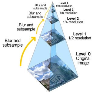
• 均值金字塔：2*2邻域均值滤波
• 高斯金字塔：向下降采样图像(4层)，高斯核5*5
• 拉普拉斯金字塔

Feature Matching

相似度

• SSD (Sum of Squared Distance)

$${D(I_A,I_B)}_{SSD}=\sum _{x,y}[I_A(x,y)-I_B(x,y){]}^2$$

• SAD (Sum of Absolute Difference)

$${D(I_A,I_B)}_{SAD}=\sum _{x,y}|I_A(x,y)-I_B(x,y)|$$

• NCC (Normalized Cross Correlation)

$${D(I_A,I_B)}_{NCC}=\frac{{\sum }_{x,y}{I}_A(x,y)I_B(x,y)}{\sqrt{{\sum }_{x,y}{I}_A(x,y{)}^2{\sum }_{x,y}{I}_B(x,y{)}^2}}$$

• 去均值 版本

块匹配

• 假设图像I1和图像I2，分别对应的角点为p1i和p2j，在图像I2角点中找到与图像I1对应的角点；
• 以角点p1i为中心，在图像I1中提取9*9的像素块作为模板图像T1i；
• 在图像I2中p1i点周围(以角点p1i为中心20*20的像素 范围)查找所有的角点p2jm(m<=n,n为该范围内角点数)；
• 遍历所有的角点p2jm，以角点p2jm为中心，在图像I2中提取9*9的像素块，计算该像素块与T1i的SSD；
• SSD最小对应的角点p2jm，即为图像I2中与图像I1中角点p1i对应的匹配角点；
• 循环执行以上5步，查找图像I2中与图像I1对应的所有匹配角点；

描述子匹配

Brute-Force

FLANN

这篇关于图像分析之图像特征点及匹配的文章就介绍到这儿，希望我们推荐的文章对编程师们有所帮助！

---