本文主要是介绍政安晨:【Keras机器学习示例演绎】(二十九)—— 利用卷积 LSTM 进行下一帧视频预测,希望对大家解决编程问题提供一定的参考价值,需要的开发者们随着小编来一起学习吧!
目录
简介
设置
数据集构建
数据可视化
模型构建
模型训练
帧预测可视化
预测视频
政安晨的个人主页:政安晨
欢迎 👍点赞✍评论⭐收藏
收录专栏: TensorFlow与Keras机器学习实战
希望政安晨的博客能够对您有所裨益,如有不足之处,欢迎在评论区提出指正!
本文目标:如何建立和训练用于下一帧视频预测的卷积 LSTM 模型。
简介
卷积 LSTM 架构通过在 LSTM 层中引入卷积递归单元,将时间序列处理和计算机视觉结合在一起。在本示例中,我们将探讨卷积 LSTM 模型在下一帧预测中的应用,下一帧预测是指在一系列过去帧的基础上预测下一个视频帧的过程。
设置
import numpy as np
import matplotlib.pyplot as pltimport keras
from keras import layersimport io
import imageio
from IPython.display import Image, display
from ipywidgets import widgets, Layout, HBox
数据集构建
在本例中,我们将使用移动 MNIST 数据集。
我们将下载该数据集,然后构建并预处理训练集和验证集。
对于下一帧预测,我们的模型将使用前一帧(我们称之为 f_n)来预测新一帧(称之为 f_(n + 1))。为了让模型能够创建这些预测,我们需要处理数据,使输入和输出 "移位",其中输入数据为帧 x_n,用于预测帧 y_(n + 1)。
# Download and load the dataset.
fpath = keras.utils.get_file("moving_mnist.npy","http://www.cs.toronto.edu/~nitish/unsupervised_video/mnist_test_seq.npy",
)
dataset = np.load(fpath)# Swap the axes representing the number of frames and number of data samples.
dataset = np.swapaxes(dataset, 0, 1)
# We'll pick out 1000 of the 10000 total examples and use those.
dataset = dataset[:1000, ...]
# Add a channel dimension since the images are grayscale.
dataset = np.expand_dims(dataset, axis=-1)# Split into train and validation sets using indexing to optimize memory.
indexes = np.arange(dataset.shape[0])
np.random.shuffle(indexes)
train_index = indexes[: int(0.9 * dataset.shape[0])]
val_index = indexes[int(0.9 * dataset.shape[0]) :]
train_dataset = dataset[train_index]
val_dataset = dataset[val_index]# Normalize the data to the 0-1 range.
train_dataset = train_dataset / 255
val_dataset = val_dataset / 255# We'll define a helper function to shift the frames, where
# `x` is frames 0 to n - 1, and `y` is frames 1 to n.
def create_shifted_frames(data):x = data[:, 0 : data.shape[1] - 1, :, :]y = data[:, 1 : data.shape[1], :, :]return x, y# Apply the processing function to the datasets.
x_train, y_train = create_shifted_frames(train_dataset)
x_val, y_val = create_shifted_frames(val_dataset)# Inspect the dataset.
print("Training Dataset Shapes: " + str(x_train.shape) + ", " + str(y_train.shape))
print("Validation Dataset Shapes: " + str(x_val.shape) + ", " + str(y_val.shape))
演绎展示:
Downloading data from http://www.cs.toronto.edu/~nitish/unsupervised_video/mnist_test_seq.npy819200096/819200096 ━━━━━━━━━━━━━━━━━━━━ 116s 0us/step
Training Dataset Shapes: (900, 19, 64, 64, 1), (900, 19, 64, 64, 1)
Validation Dataset Shapes: (100, 19, 64, 64, 1), (100, 19, 64, 64, 1)
数据可视化
我们的数据由一系列的帧组成,每个帧都用于预测即将到来的帧。让我们来看一些这些连续帧。
# Construct a figure on which we will visualize the images.
fig, axes = plt.subplots(4, 5, figsize=(10, 8))# Plot each of the sequential images for one random data example.
data_choice = np.random.choice(range(len(train_dataset)), size=1)[0]
for idx, ax in enumerate(axes.flat):ax.imshow(np.squeeze(train_dataset[data_choice][idx]), cmap="gray")ax.set_title(f"Frame {idx + 1}")ax.axis("off")# Print information and display the figure.
print(f"Displaying frames for example {data_choice}.")
plt.show()
Displaying frames for example 95.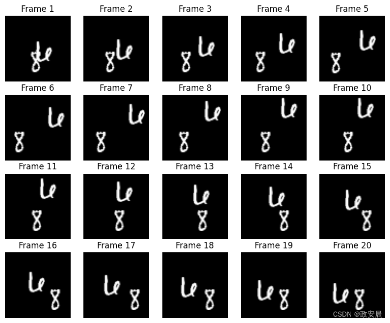
模型构建
为了构建一个卷积LSTM模型,我们将使用ConvLSTM2D层,该层将接受形状为(batch_size,num_frames,width,height,channels)的输入,并返回相同形状的预测电影。
# Construct the input layer with no definite frame size.
inp = layers.Input(shape=(None, *x_train.shape[2:]))# We will construct 3 `ConvLSTM2D` layers with batch normalization,
# followed by a `Conv3D` layer for the spatiotemporal outputs.
x = layers.ConvLSTM2D(filters=64,kernel_size=(5, 5),padding="same",return_sequences=True,activation="relu",
)(inp)
x = layers.BatchNormalization()(x)
x = layers.ConvLSTM2D(filters=64,kernel_size=(3, 3),padding="same",return_sequences=True,activation="relu",
)(x)
x = layers.BatchNormalization()(x)
x = layers.ConvLSTM2D(filters=64,kernel_size=(1, 1),padding="same",return_sequences=True,activation="relu",
)(x)
x = layers.Conv3D(filters=1, kernel_size=(3, 3, 3), activation="sigmoid", padding="same"
)(x)# Next, we will build the complete model and compile it.
model = keras.models.Model(inp, x)
model.compile(loss=keras.losses.binary_crossentropy,optimizer=keras.optimizers.Adam(),
)
模型训练
有了模型和数据,我们就可以训练模型了。
# Define some callbacks to improve training.
early_stopping = keras.callbacks.EarlyStopping(monitor="val_loss", patience=10)
reduce_lr = keras.callbacks.ReduceLROnPlateau(monitor="val_loss", patience=5)# Define modifiable training hyperparameters.
epochs = 20
batch_size = 5# Fit the model to the training data.
model.fit(x_train,y_train,batch_size=batch_size,epochs=epochs,validation_data=(x_val, y_val),callbacks=[early_stopping, reduce_lr],
)
演绎展示:
Epoch 1/20180/180 ━━━━━━━━━━━━━━━━━━━━ 50s 226ms/step - loss: 0.1510 - val_loss: 0.2966 - learning_rate: 0.0010
Epoch 2/20180/180 ━━━━━━━━━━━━━━━━━━━━ 40s 219ms/step - loss: 0.0287 - val_loss: 0.1766 - learning_rate: 0.0010
Epoch 3/20180/180 ━━━━━━━━━━━━━━━━━━━━ 40s 219ms/step - loss: 0.0269 - val_loss: 0.0661 - learning_rate: 0.0010
Epoch 4/20180/180 ━━━━━━━━━━━━━━━━━━━━ 40s 219ms/step - loss: 0.0264 - val_loss: 0.0279 - learning_rate: 0.0010
Epoch 5/20180/180 ━━━━━━━━━━━━━━━━━━━━ 40s 219ms/step - loss: 0.0258 - val_loss: 0.0254 - learning_rate: 0.0010
Epoch 6/20180/180 ━━━━━━━━━━━━━━━━━━━━ 40s 219ms/step - loss: 0.0256 - val_loss: 0.0253 - learning_rate: 0.0010
Epoch 7/20180/180 ━━━━━━━━━━━━━━━━━━━━ 40s 219ms/step - loss: 0.0251 - val_loss: 0.0248 - learning_rate: 0.0010
Epoch 8/20180/180 ━━━━━━━━━━━━━━━━━━━━ 40s 219ms/step - loss: 0.0251 - val_loss: 0.0251 - learning_rate: 0.0010
Epoch 9/20180/180 ━━━━━━━━━━━━━━━━━━━━ 40s 219ms/step - loss: 0.0247 - val_loss: 0.0243 - learning_rate: 0.0010
Epoch 10/20180/180 ━━━━━━━━━━━━━━━━━━━━ 40s 219ms/step - loss: 0.0246 - val_loss: 0.0246 - learning_rate: 0.0010
Epoch 11/20180/180 ━━━━━━━━━━━━━━━━━━━━ 40s 219ms/step - loss: 0.0245 - val_loss: 0.0247 - learning_rate: 0.0010
Epoch 12/20180/180 ━━━━━━━━━━━━━━━━━━━━ 40s 219ms/step - loss: 0.0241 - val_loss: 0.0243 - learning_rate: 0.0010
Epoch 13/20180/180 ━━━━━━━━━━━━━━━━━━━━ 40s 219ms/step - loss: 0.0244 - val_loss: 0.0245 - learning_rate: 0.0010
Epoch 14/20180/180 ━━━━━━━━━━━━━━━━━━━━ 40s 219ms/step - loss: 0.0241 - val_loss: 0.0241 - learning_rate: 0.0010
Epoch 15/20180/180 ━━━━━━━━━━━━━━━━━━━━ 40s 219ms/step - loss: 0.0243 - val_loss: 0.0241 - learning_rate: 0.0010
Epoch 16/20180/180 ━━━━━━━━━━━━━━━━━━━━ 40s 219ms/step - loss: 0.0242 - val_loss: 0.0242 - learning_rate: 0.0010
Epoch 17/20180/180 ━━━━━━━━━━━━━━━━━━━━ 40s 219ms/step - loss: 0.0240 - val_loss: 0.0240 - learning_rate: 0.0010
Epoch 18/20180/180 ━━━━━━━━━━━━━━━━━━━━ 40s 219ms/step - loss: 0.0240 - val_loss: 0.0243 - learning_rate: 0.0010
Epoch 19/20180/180 ━━━━━━━━━━━━━━━━━━━━ 40s 219ms/step - loss: 0.0240 - val_loss: 0.0244 - learning_rate: 0.0010
Epoch 20/20180/180 ━━━━━━━━━━━━━━━━━━━━ 40s 219ms/step - loss: 0.0237 - val_loss: 0.0238 - learning_rate: 1.0000e-04<keras.src.callbacks.history.History at 0x7ff294f9c340>
帧预测可视化
在构建并训练好模型后,我们可以根据新视频生成一些帧预测示例。
我们将从验证集中随机挑选一个示例,然后从中选择前十个帧。在此基础上,我们可以让模型预测 10 个新帧,并将其与地面实况帧预测进行比较。
# Select a random example from the validation dataset.
example = val_dataset[np.random.choice(range(len(val_dataset)), size=1)[0]]# Pick the first/last ten frames from the example.
frames = example[:10, ...]
original_frames = example[10:, ...]# Predict a new set of 10 frames.
for _ in range(10):# Extract the model's prediction and post-process it.new_prediction = model.predict(np.expand_dims(frames, axis=0))new_prediction = np.squeeze(new_prediction, axis=0)predicted_frame = np.expand_dims(new_prediction[-1, ...], axis=0)# Extend the set of prediction frames.frames = np.concatenate((frames, predicted_frame), axis=0)# Construct a figure for the original and new frames.
fig, axes = plt.subplots(2, 10, figsize=(20, 4))# Plot the original frames.
for idx, ax in enumerate(axes[0]):ax.imshow(np.squeeze(original_frames[idx]), cmap="gray")ax.set_title(f"Frame {idx + 11}")ax.axis("off")# Plot the new frames.
new_frames = frames[10:, ...]
for idx, ax in enumerate(axes[1]):ax.imshow(np.squeeze(new_frames[idx]), cmap="gray")ax.set_title(f"Frame {idx + 11}")ax.axis("off")# Display the figure.
plt.show()
1/1 ━━━━━━━━━━━━━━━━━━━━ 2s 2s/step1/1 ━━━━━━━━━━━━━━━━━━━━ 1s 800ms/step1/1 ━━━━━━━━━━━━━━━━━━━━ 1s 805ms/step1/1 ━━━━━━━━━━━━━━━━━━━━ 1s 790ms/step1/1 ━━━━━━━━━━━━━━━━━━━━ 1s 821ms/step1/1 ━━━━━━━━━━━━━━━━━━━━ 1s 824ms/step1/1 ━━━━━━━━━━━━━━━━━━━━ 1s 928ms/step1/1 ━━━━━━━━━━━━━━━━━━━━ 1s 813ms/step1/1 ━━━━━━━━━━━━━━━━━━━━ 1s 810ms/step1/1 ━━━━━━━━━━━━━━━━━━━━ 1s 814ms/step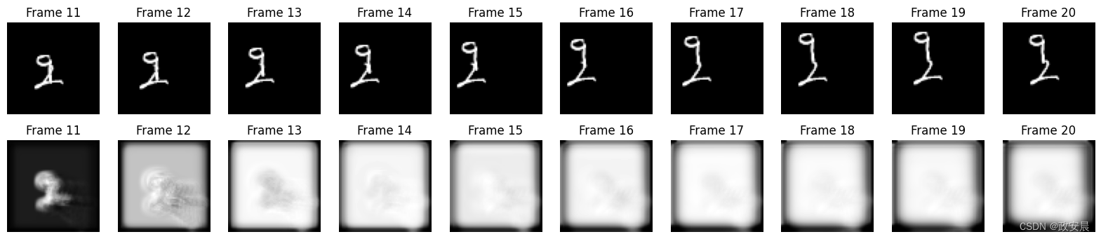
预测视频
最后,我们将从验证集中挑选几个例子,用它们制作一些 GIF,看看模型预测的视频。
你可以使用 Hugging Face Hub 上托管的训练有素的模型,也可以在 Hugging Face Spaces 上尝试演示。
# Select a few random examples from the dataset.
examples = val_dataset[np.random.choice(range(len(val_dataset)), size=5)]# Iterate over the examples and predict the frames.
predicted_videos = []
for example in examples:# Pick the first/last ten frames from the example.frames = example[:10, ...]original_frames = example[10:, ...]new_predictions = np.zeros(shape=(10, *frames[0].shape))# Predict a new set of 10 frames.for i in range(10):# Extract the model's prediction and post-process it.frames = example[: 10 + i + 1, ...]new_prediction = model.predict(np.expand_dims(frames, axis=0))new_prediction = np.squeeze(new_prediction, axis=0)predicted_frame = np.expand_dims(new_prediction[-1, ...], axis=0)# Extend the set of prediction frames.new_predictions[i] = predicted_frame# Create and save GIFs for each of the ground truth/prediction images.for frame_set in [original_frames, new_predictions]:# Construct a GIF from the selected video frames.current_frames = np.squeeze(frame_set)current_frames = current_frames[..., np.newaxis] * np.ones(3)current_frames = (current_frames * 255).astype(np.uint8)current_frames = list(current_frames)# Construct a GIF from the frames.with io.BytesIO() as gif:imageio.mimsave(gif, current_frames, "GIF", duration=200)predicted_videos.append(gif.getvalue())# Display the videos.
print(" Truth\tPrediction")
for i in range(0, len(predicted_videos), 2):# Construct and display an `HBox` with the ground truth and prediction.box = HBox([widgets.Image(value=predicted_videos[i]),widgets.Image(value=predicted_videos[i + 1]),])display(box)
1/1 ━━━━━━━━━━━━━━━━━━━━ 0s 6ms/step1/1 ━━━━━━━━━━━━━━━━━━━━ 0s 5ms/step1/1 ━━━━━━━━━━━━━━━━━━━━ 0s 5ms/step1/1 ━━━━━━━━━━━━━━━━━━━━ 0s 5ms/step1/1 ━━━━━━━━━━━━━━━━━━━━ 0s 6ms/step1/1 ━━━━━━━━━━━━━━━━━━━━ 0s 6ms/step1/1 ━━━━━━━━━━━━━━━━━━━━ 0s 8ms/step1/1 ━━━━━━━━━━━━━━━━━━━━ 0s 7ms/step1/1 ━━━━━━━━━━━━━━━━━━━━ 0s 7ms/step1/1 ━━━━━━━━━━━━━━━━━━━━ 1s 790ms/step1/1 ━━━━━━━━━━━━━━━━━━━━ 0s 5ms/step1/1 ━━━━━━━━━━━━━━━━━━━━ 0s 5ms/step1/1 ━━━━━━━━━━━━━━━━━━━━ 0s 5ms/step1/1 ━━━━━━━━━━━━━━━━━━━━ 0s 5ms/step1/1 ━━━━━━━━━━━━━━━━━━━━ 0s 6ms/step1/1 ━━━━━━━━━━━━━━━━━━━━ 0s 6ms/step1/1 ━━━━━━━━━━━━━━━━━━━━ 0s 7ms/step1/1 ━━━━━━━━━━━━━━━━━━━━ 0s 7ms/step1/1 ━━━━━━━━━━━━━━━━━━━━ 0s 8ms/step1/1 ━━━━━━━━━━━━━━━━━━━━ 0s 8ms/step1/1 ━━━━━━━━━━━━━━━━━━━━ 0s 6ms/step1/1 ━━━━━━━━━━━━━━━━━━━━ 0s 6ms/step1/1 ━━━━━━━━━━━━━━━━━━━━ 0s 5ms/step1/1 ━━━━━━━━━━━━━━━━━━━━ 0s 6ms/step1/1 ━━━━━━━━━━━━━━━━━━━━ 0s 6ms/step1/1 ━━━━━━━━━━━━━━━━━━━━ 0s 6ms/step1/1 ━━━━━━━━━━━━━━━━━━━━ 0s 7ms/step1/1 ━━━━━━━━━━━━━━━━━━━━ 0s 7ms/step1/1 ━━━━━━━━━━━━━━━━━━━━ 0s 7ms/step1/1 ━━━━━━━━━━━━━━━━━━━━ 0s 8ms/step1/1 ━━━━━━━━━━━━━━━━━━━━ 0s 6ms/step1/1 ━━━━━━━━━━━━━━━━━━━━ 0s 5ms/step1/1 ━━━━━━━━━━━━━━━━━━━━ 0s 6ms/step1/1 ━━━━━━━━━━━━━━━━━━━━ 0s 6ms/step1/1 ━━━━━━━━━━━━━━━━━━━━ 0s 7ms/step1/1 ━━━━━━━━━━━━━━━━━━━━ 0s 8ms/step1/1 ━━━━━━━━━━━━━━━━━━━━ 0s 6ms/step1/1 ━━━━━━━━━━━━━━━━━━━━ 0s 7ms/step1/1 ━━━━━━━━━━━━━━━━━━━━ 0s 7ms/step1/1 ━━━━━━━━━━━━━━━━━━━━ 0s 9ms/step1/1 ━━━━━━━━━━━━━━━━━━━━ 0s 5ms/step1/1 ━━━━━━━━━━━━━━━━━━━━ 0s 5ms/step1/1 ━━━━━━━━━━━━━━━━━━━━ 0s 5ms/step1/1 ━━━━━━━━━━━━━━━━━━━━ 0s 5ms/step1/1 ━━━━━━━━━━━━━━━━━━━━ 0s 6ms/step1/1 ━━━━━━━━━━━━━━━━━━━━ 0s 6ms/step1/1 ━━━━━━━━━━━━━━━━━━━━ 0s 6ms/step1/1 ━━━━━━━━━━━━━━━━━━━━ 0s 7ms/step1/1 ━━━━━━━━━━━━━━━━━━━━ 0s 8ms/step1/1 ━━━━━━━━━━━━━━━━━━━━ 0s 10ms/stepTruth PredictionHBox(children=(Image(value=b'GIF89a@\x00@\x00\x87\x00\x00\xff\xff\xff\xfe\xfe\xfe\xfd\xfd\xfd\xfc\xfc\xfc\xf8\…HBox(children=(Image(value=b'GIF89a@\x00@\x00\x86\x00\x00\xff\xff\xff\xfd\xfd\xfd\xfc\xfc\xfc\xfb\xfb\xfb\xf4\…HBox(children=(Image(value=b'GIF89a@\x00@\x00\x86\x00\x00\xff\xff\xff\xfe\xfe\xfe\xfd\xfd\xfd\xfc\xfc\xfc\xfb\…HBox(children=(Image(value=b'GIF89a@\x00@\x00\x86\x00\x00\xff\xff\xff\xfe\xfe\xfe\xfd\xfd\xfd\xfc\xfc\xfc\xfb\…HBox(children=(Image(value=b'GIF89a@\x00@\x00\x86\x00\x00\xff\xff\xff\xfd\xfd\xfd\xfc\xfc\xfc\xf9\xf9\xf9\xf7\…这篇关于政安晨:【Keras机器学习示例演绎】(二十九)—— 利用卷积 LSTM 进行下一帧视频预测的文章就介绍到这儿,希望我们推荐的文章对编程师们有所帮助!


