【信号处理】基于变分自编码器（VAE）的图片典型增强方法实现

本文主要是介绍【信号处理】基于变分自编码器（VAE）的图片典型增强方法实现，希望对大家解决编程问题提供一定的参考价值，需要的开发者们随着小编来一起学习吧！

关于

深度学习中，经常面临图片数据量较小的问题，此时，对数据进行增强，显得比较重要。传统的图片增强方法包括剪切，增加噪声，改变对比度等等方法，但是，对于后端任务的性能提升有限。所以，变分自编码器被用来实现深度数据增强。

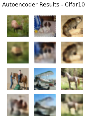
变分自编码器的主要缺点在于生成图像过于平滑和模糊，图像细节重建不足。

常见的图像增强方法：https://www.tensorflow.org/tutorials/images/data_augmentation

工具

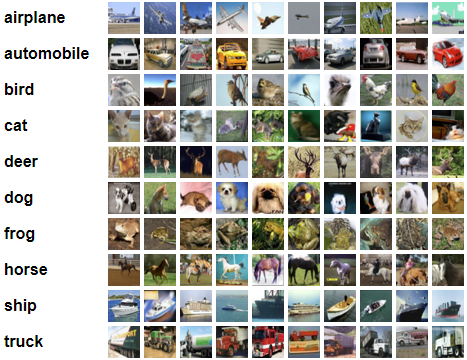
数据集下载地址： CIFAR-10 and CIFAR-100 datasets

方法实现

加载数据和必要的库函数

import tensorflow.compat.v1.keras.backend as K
import tensorflow as tf
tf.compat.v1.disable_eager_execution()
import matplotlib.pyplot as plt
import numpy as np
from numpy import random
import tensorflow_datasets as tfds
import keras
from keras.models import Model
from keras.layers import Conv2D, Conv2DTranspose, Input, Flatten, Dense, Lambda, Reshapextrain , ytrain = tfds.as_numpy(tfds.load('cifar10',split='train',batch_size=-1,as_supervised=True,))
xtest , ytest = tfds.as_numpy(tfds.load('cifar10',split='test',batch_size=-1,as_supervised=True,))
xtrain = (xtrain.astype('float32'))/255
xtest = (xtest.astype('float32'))/255height=32
width=32
channels=3
print(f"Train Shape: {xtrain.shape},Test Shape: {xtest.shape}")
plt.imshow(xtrain[0])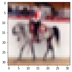

编码器模型搭建

input_shape=(height,width,channels)
latent_dims=3072input_img= Input(shape=input_shape, name='encoder_input')
x=Conv2D(128, 4, padding='same', activation='relu',strides=2)(input_img)
x=Conv2D(256, 4, padding='same', activation='relu',strides=2)(x)
x=Conv2D(512, 4, padding='same', activation='relu',strides=2)(x)
x=Conv2D(1024, 4, padding='same', activation='relu',strides=2)(x)
conv_shape = K.int_shape(x)
x=Flatten()(x)
x=Dense(3072, activation='relu')(x)
z_mean=Dense(latent_dims, name='latent_mean')(x)
z_sigma=Dense(latent_dims, name='latent_sigma')(x)def sampler(args):z_mean, z_sigma = argseps = K.random_normal(shape=(K.shape(z_mean)[0], K.int_shape(z_mean)[1]))return z_mean + K.exp(z_sigma / 2) * epsz = Lambda(sampler, output_shape=(latent_dims, ), name='z')([z_mean, z_sigma])encoder = Model(input_img, [z_mean, z_sigma, z], name='encoder')
print(encoder.summary())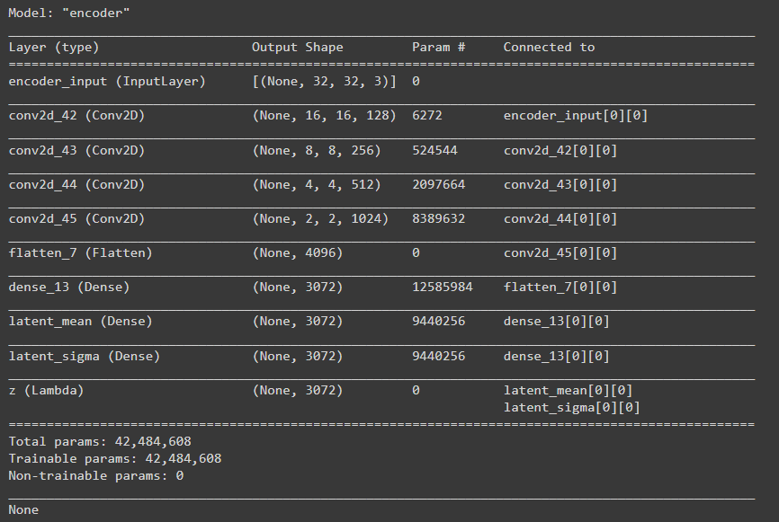

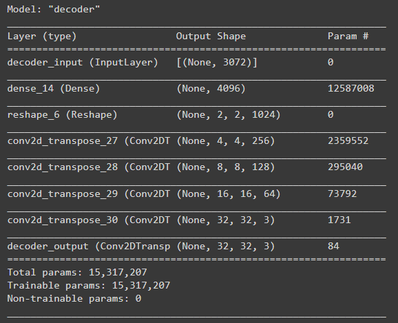
解码器模型构建

decoder_input = Input(shape=(latent_dims, ), name='decoder_input')
x = Dense(conv_shape[1]*conv_shape[2]*conv_shape[3], activation='relu')(decoder_input)
x = Reshape((conv_shape[1], conv_shape[2], conv_shape[3]))(x)
x = Conv2DTranspose(256, 3, padding='same', activation='relu',strides=(2, 2))(x)
x = Conv2DTranspose(128, 3, padding='same', activation='relu',strides=(2, 2))(x)
x = Conv2DTranspose(64, 3, padding='same', activation='relu',strides=(2, 2))(x)
x = Conv2DTranspose(3, 3, padding='same', activation='relu',strides=(2, 2))(x)
x = Conv2DTranspose(channels, 3, padding='same', activation='sigmoid', name='decoder_output')(x)
decoder = Model(decoder_input, x, name='decoder')
decoder.summary()
z_decoded = decoder(z)class CustomLayer(keras.layers.Layer):def vae_loss(self, x, z_decoded):x = K.flatten(x)z_decoded = K.flatten(z_decoded)# Reconstruction loss (as we used sigmoid activation we can use binarycrossentropy)recon_loss = keras.metrics.binary_crossentropy(x, z_decoded)# KL divergencekl_loss = -5e-4 * K.mean(1 + z_sigma - K.square(z_mean) - K.exp(z_sigma), axis=-1)return K.mean(recon_loss + kl_loss)# add custom loss to the classdef call(self, inputs):x = inputs[0]z_decoded = inputs[1]loss = self.vae_loss(x, z_decoded)self.add_loss(loss, inputs=inputs)return x

整体模型构建

y = CustomLayer()([input_img, z_decoded])vae = Model(input_img, y, name='vae')
vae.compile(optimizer='adam', loss=None)
vae.summary()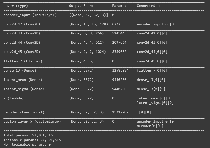

模型训练

history=vae.fit(xtrain, verbose=2, epochs = 100, batch_size = 64, validation_split = 0.2)

训练可视化

f = plt.figure(figsize=(10,7))
f.add_subplot()
#Adding Subplot
plt.plot(history.epoch, history.history['loss'], label = "loss") # Loss curve for training set
plt.plot(history.epoch, history.history['val_loss'], label = "val_loss") # Loss curve for validation setplt.title("Loss Curve",fontsize=18)
plt.xlabel("Epochs",fontsize=15)
plt.ylabel("Loss",fontsize=15)
plt.grid(alpha=0.3)
plt.legend()
plt.savefig("VAE_Loss_Trial5.png")
plt.show()

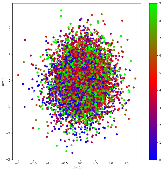
中间编码特征可视化

mu, _, _ = encoder.predict(xtest)
#Plot dim1 and dim2 for mu
plt.figure(figsize=(10, 10))
plt.scatter(mu[:, 0], mu[:, 1], c=ytest, cmap='brg')
plt.xlabel('dim 1')
plt.ylabel('dim 2')
plt.colorbar()
plt.show()
plt.savefig("VAE_Colourbar_Trial5.png")

数据增强生成

#RANDOM GENERATION
def generate():n=20figure = np.zeros((width *2 , height * 10, channels))#Create a Grid of latent variables, to be provided as inputs to decoder.predict
#Creating vectors within range -5 to 5 as that seems to be the range in latent spacefor k in range(2):for l in range(10):z_sample =random.rand(3072)z_out=np.array([z_sample])x_decoded = decoder.predict(z_out)digit = x_decoded[0].reshape(width, height, channels)figure[k * width: (k + 1) * width,l * height: (l + 1) * height] = digitplt.figure(figsize=(10, 10))
#Reshape for visualizationfig_shape = np.shape(figure)figure = figure.reshape((fig_shape[0], fig_shape[1],3))plt.imshow(figure, cmap='gnuplot2')plt.show()  plt.savefig("VAE_imagesgen_Trial5.png")

解码器图像重建

#IMAGE RECONSTRUCT USING TEST SET IMGS
def reconstruct():num_imgs = 6rand = np.random.randint(1, xtest.shape[0]-6) xtestsample = xtest[rand:rand+num_imgs]x_encoded = np.array(encoder.predict(xtestsample))latent_xtest=x_encoded[2]x_decoded = decoder.predict(latent_xtest)rows = 2 # defining no. of rows in figurecols = 3 # defining no. of colums in figurecell_size = 1.5f = plt.figure(figsize=(cell_size*cols,cell_size*rows*2)) # defining a figure f.tight_layout()for i in range(rows):for j in range(cols): f.add_subplot(rows*2,cols, (2*i*cols)+(j+1)) # adding sub plot to figure on each iterationplt.imshow(xtestsample[i*cols + j]) plt.axis("off")for j in range(cols): f.add_subplot(rows*2,cols,((2*i+1)*cols)+(j+1)) # adding sub plot to figure on each iterationplt.imshow(x_decoded[i*cols + j]) plt.axis("off")f.suptitle("Autoencoder Results - Cifar10",fontsize=18)plt.savefig("VAE_imagesrecons_Trial5.png")plt.show()