MATLAB：符号运算

本文主要是介绍MATLAB：符号运算，希望对大家解决编程问题提供一定的参考价值，需要的开发者们随着小编来一起学习吧！

一、符号运算简介与符号定义

见PPT

二、符号表达式的化简与替换

见PPT

三、符号函数图形绘制

 

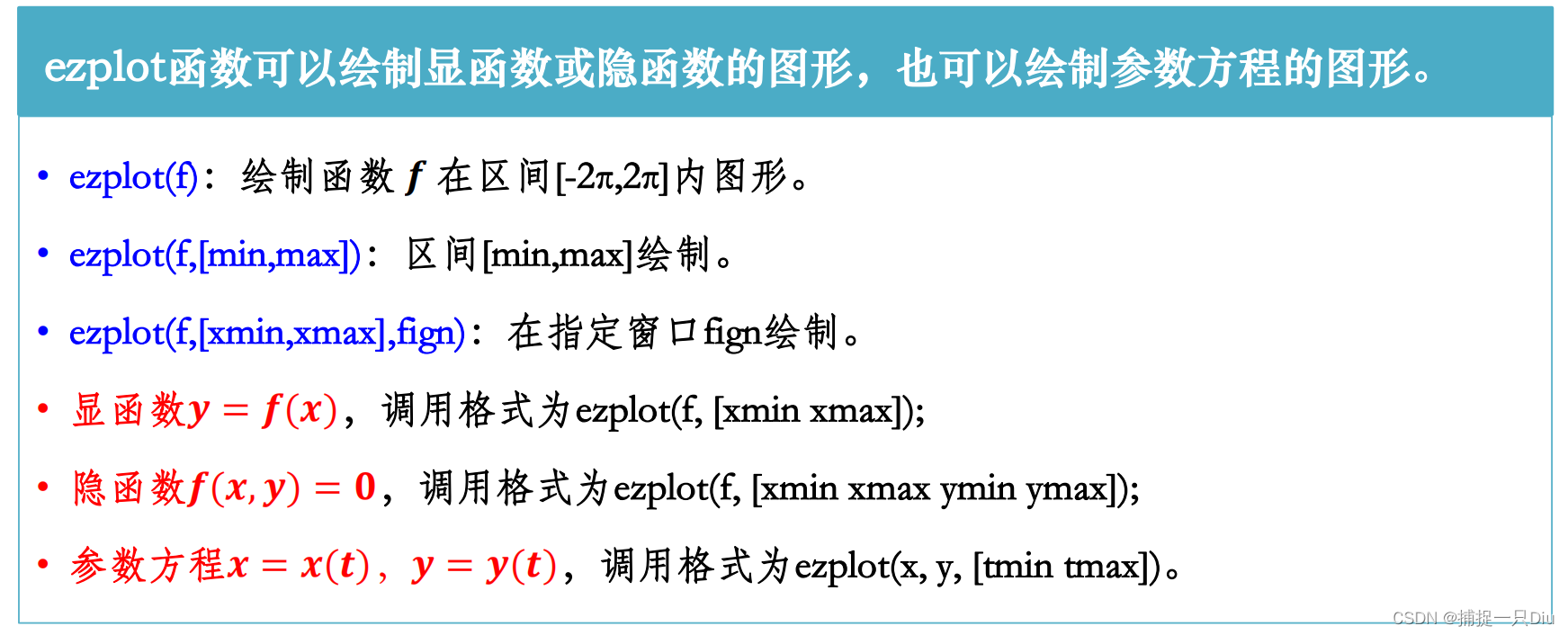
syms x
fh1 = (x^2+sin(2*x))/5;
fh2 = 3/8*(exp(-2*x/3)*sin(1+2*x));
h1 = ezplot(fh1,[-5,5]);
set(h1,{'LineWidth','LineStyle','Color'},{1.3,'--','r'})
grid on
hold on
h2 = ezplot(fh2,[-5,5]);
set(h2,{'LineWidth','LineStyle','Color'},{1.3,'-.','b'})
axis([-5,5,-3.5,3.5])
legend('fh1 = x^2*sin(2*x)/5','fh2 = 3/8*(exp(-2*x/3)*sin(1+2*x))')
legend('boxoff')

syms x y
fh = x^2*sin(x+y^2)+y^2*exp(x)+6*cos(x^2+y);
h = ezplot(fh,[-6 6]);
set(h,{'LineWidth','LineStyle','Color'},{1,'-','b'})
grid on

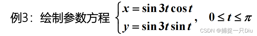
syms t
x = sin(3*t)*cos(t);
y = sin(3*t)*sin(t);
h = ezplot(x,y,[0,pi]);
set(h,'linewidth',1.3,'linestyle','-.','color','r')
grid on

syms t
x = cos(t);
y = sin(t); 
z = t; 
subplot(2,1,1)
ezplot3(x,y,z,[0,6*pi],'animate');
subplot(2,1,2)
h1 = ezplot3(x,y,z,[0,2*pi]);
set(h1,'linewidth',1.3,'linestyle',':','color','r')
hold on
h2 = ezplot3(x,y,z,[2*pi,4*pi]);
set(h2,'linewidth',1.3,'linestyle','-.','color','b')
h3 = ezplot3(x,y,z,[4*pi,6*pi]);
set(h3,'linewidth',1.3,'linestyle','--','color','c')

syms x y
z = x*exp(-x^2-y^2);
subplot(2,2,1)
ezmesh(z,[-2.5,2.5],30);
subplot(2,2,2)
ezsurf(z,[-2.5,2.5],30);
subplot(2,2,3)
ezmesh(z,[-2.5,2.5],60);
subplot(2,2,4)
ezsurf(z,[-2.5,2.5],60);
shading interp

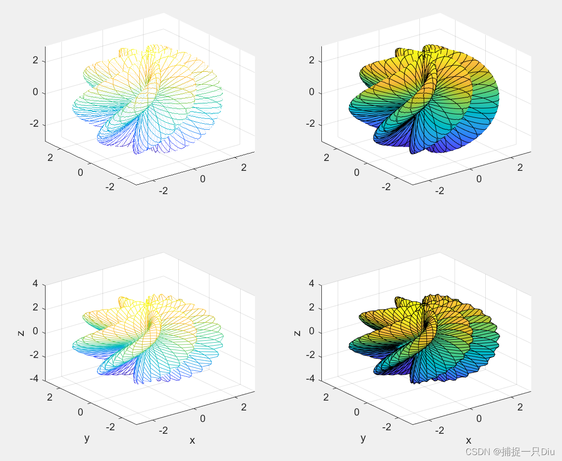
r = @(s,t) 2 + sin(7.*s + 5.*t);
x = @(s,t) r(s,t).*cos(s).*sin(t);
y = @(s,t) r(s,t).*sin(s).*sin(t);
z = @(s,t) r(s,t).*cos(t); 
subplot(2,2,1)
fmesh(x,y,z,[0 2*pi 0 pi])
alpha(0.8)
subplot(2,2,2)
fsurf(x,y,z,[0 2*pi 0 pi])
x = sym(x);
y = sym(y);
z = sym(z);
subplot(2,2,3)
ezmesh(x,y,z,[0,2*pi,0,pi])
subplot(2,2,4)
ezsurf(x,y,z,[0,2*pi,0,pi])

syms x y
fh = y/(1 + x^2 + y^2);
subplot(2,2,1)
ezmeshc(fh,[-5,5,-2*pi,2*pi],30)
subplot(2,2,2)
ezsurfc(fh,[-5,5,-2*pi,2*pi],30),
%fmesh和fsurf函数实现同样的绘图效果
subplot(2,2,3)
fmesh(fh,[-5,5,-2*pi,2*pi],'ShowContours','on')
subplot(2,2,4)
fsurf(fh,[-5,5,-2*pi,2*pi],'ShowContours','on')

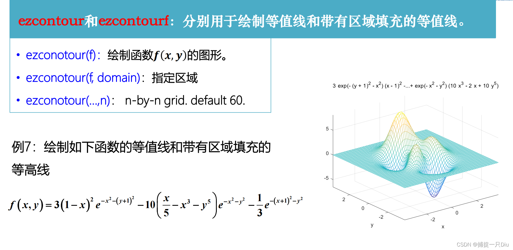
syms x y
fh = 3*(1-x)^2*exp(-(x^2)-(y+1)^2)-10*(x/5 - x^3 - y^5)*exp(-x^2-y^2)-1/3*exp(-(x+1)^2 - y^2);
% ezmesh(fh)
subplot(1,2,1)
ezcontour(fh,[-3,3],49)
title('ezcoutour函数绘制等高线')
subplot(1,2,2),
ezcontourf(fh,[-3,3],49)
title('ezcoutourf函数绘制带有区域填充的等高线')
figure
subplot(1,2,1)
fcontour(fh)
set(gca,'XTick',-5:1:5)
subplot(1,2,2)
fcontour(fh,'Fill','on')
set(gca,'XTick',-5:1:5)

四、符号表达式求极限

syms x a b n y
fh1 = x*(1+a/x)^x*sin(b/x);
lim1 = limit(fh1,x,inf)fh2 = (exp(x^3)-1)/(1-cos(sqrt(x-sin(x))));
lim2 = limit(fh2,x,0,'right')fh3 = n^(2/3)*sin(factorial(n))/(n+1);
lim3 = limit(fh3,n,inf)fh4 = n*atan(1/(n*(x^2+1)+x))*(tan(pi/4+x/(2*n)))^n;
lim4 = limit(fh4,n,inf)fh5 = exp(-1/(y^2+x^2))*(sin(x))^2/x^2*(1+1/y^2)^(x+a^2*y^2);
% lim5 = limit(limit(fh5,x,1/sqrt(y)),y,inf) 无法求解
fh5 = subs(fh5,x,1/sqrt(y));
lim5 = limit(fh5,y,inf)

 

fh6 = (x^(1/3)+y)*sin(1/x)*cos(1/y);
% lim6 = limit(limit(fh6,x,0),y,0) 无法求解
lim6 = limit(limit(fh6,x,1e-25),y,1e-25)
vpa(lim6)

 五、符号微分

syms a b t x y z
fh1 = sqrt(1+exp(x));
df1 = diff(fh1)fh2 = x*cos(x); 
df2 = diff(fh2,x,2) 
df23 = diff(fh2,x,3) ft1 = a*cos(t); 
ft2 = b*sin(t);
df3 = diff(ft2)/diff(ft1)
df32 = diff(df3,t)/diff(ft1,t)
% df32 = (diff(ft1)*diff(ft2,2)-diff(ft1,2)*diff(ft2))/(diff(ft1))^3 fh4 = x*exp(y)/y^2;
df4x = diff(fh4,x) 
df4y = diff(fh4,y) fh5 = x^2+y^2+z^2-a^2;
zx = -diff(fh5,x)/diff(fh5,z)
zy = -diff(fh5,y)/diff(fh5,z) 

syms x y t
fh = sin(x^2)*y^2;
dfh1 = diff(fh,x,2)
dfh2 = diff(diff(fh,x,2),y,1)fh = sin(x)/(x^2 + 4*x + 3);
dfh4 = diff(fh,x,4)
fhs = simplify(dfh4)
fhsc = collect(fhs,'cos')
subexpr(fhsc)

syms t f(t)
Ft = t^2*f(t)*sin(t);
DFt = diff(Ft,t,3)
DFt = subs(DFt,f(t),exp(-t))
DFt = simplify(DFt)
pretty(DFt)Fts = subs(Ft,f(t),exp(-t))
Fts3 = diff(Fts,t,3)
Fts3 = simplify(Fts3)

 

syms x
H = [4*sin(5*x),exp(-4*x^2); 3*x^2+4*x+1,sqrt(4*x^2+2)]; 
H3 = diff(H,x,3)
H3 = simplify(H3)

function dy = impldiff_n(f,x,y,n)% f表示隐函数，n要求是正整数if mod(n,1) ~= 0 error('n should positive integer, please correct.')elseF1 = -simplify(diff(f,x)/diff(f,y)); % 一阶偏导dy = F1;for i = 2:n% 按递推公式编写dy = simplify(diff(dy,x) + diff(dy,y)*F1); endend
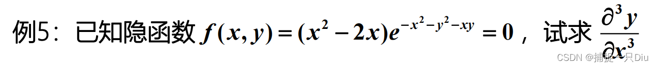
end

syms x y
fh = (x^2-2*x)*exp(-x^2-y^2-x*y);
dfh1 = impldiff_n(fh,x,y,1)
dfh3 = impldiff_n(fh,x,y,3)

function result = paradiff_n(y,x,t,n)if mod(n,1) ~= 0error('n should positive integer, please correct');elseif n == 1result = diff(y,t)/diff(x,t); else%递归调用result = diff(paradiff_n(y,x,t,n-1),t)/diff(x,t); endresult = simplify(result);
end

syms t
y = sin(t)/(t+1)^3; 
x = cos(t)/(t+1)^3; 
f1 = paradiff_n(y,x,t,1)
f2 = paradiff_n(y,x,t,3)

syms x
y1 = x^3+3*x-2;
dy1 = diff(y1,x,1);
fh = dy1 - 4;
solx = solve(fh,x);
h1 = ezplot(y1);
set(h1,{'Color','LineStyle','LineWidth'},{'r','-',1.2})
y2 = 4*x-1;
hold on
h2 = ezplot(y2);
set(h2,{'Color','LineStyle','LineWidth'},{'b','-',1.2})
fval = subs(y1,solx);
plot(solx,fval,'r.','Markersize',15)
f1 = 4*(x-solx(1))+fval(1);
f2 = 4*(x-solx(2))+fval(2);
h3 = ezplot(f1);
set(h3,{'Color','LineStyle','LineWidth'},{'k','--',1})
h4 = ezplot(f2);
set(h4,{'Color','LineStyle','LineWidth'},{'k','--',1})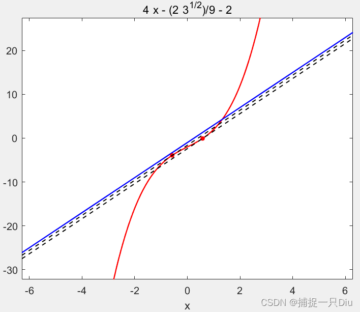

六、符号积分

 

syms x alpha t
fh1 = (3-x^2)^3;
I1 = int(fh1)fh2 = (sin(x))^2;
I2 = int(fh2)fh3 = exp(alpha*t);
I3 = int(fh3,t)fh4 = 5*x*t/(1+x^2);
I4 = int(fh4,t)fh5 = abs(1-x);
I5 = int(fh5,1,2)fh6 = 1/(1+x^2);
I6 = int(fh6,-inf,inf)fh7 = 4*x/t;
I7 = int(fh7,t,2,sin(x))fh8 = x^3/(x-1)^10;
I8 = int(fh8,2,3)

syms x y
int1 = int(int(x*sin(x),x,y,sqrt(y)),y,0,1)int2 = int(int(x*exp(-y^2),x,0,sqrt(y)),y,0,1)int3 = int(int(x^2+y^2,x,sqrt(y),2),y,1,4)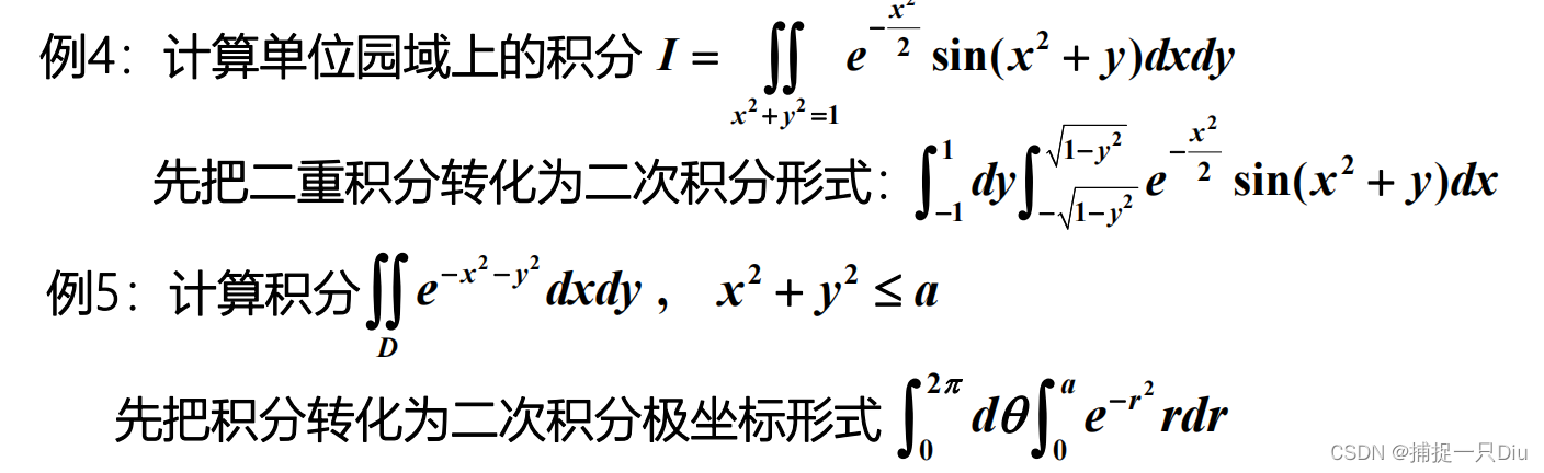

syms x y
I1 = int(int(exp(-x^2/2)*sin(x^2+y),x,-sqrt(1-y^2),sqrt(1-y^2)),y,-1,1)
vpa(I1,10)
syms theta r a
I2 = int(int(exp(-r^2)*r,r,0,a),theta,0,2*pi)fh1 = @(x,y)exp(-x.^2./2).*sin(x.^2+y);
xmin = @(y)-sqrt(1-y.^2);
xmax = @(y)sqrt(1-y.^2);
I = integral2(fh1,-1,1,xmin,xmax)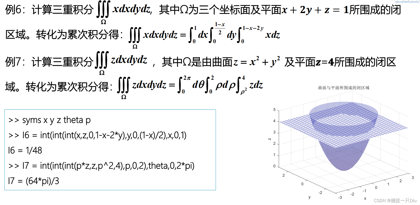

第一类曲线积分：

syms t
syms a positive
% a = syms('a'), assume(a,'positive')
x = a*cos(t);
y = a*sin(t);
z = a*t;
ds = sqrt(diff(x,t)^2 + diff(y,t)^2 + diff(z,t)^2);
fh = z^2/(x^2+y^2)*ds;
I = int(fh,t,0,2*pi)syms a t k
x = a*cos(t);
y = a*sin(t);
z = k*t;
ds = sqrt(diff(x,t)^2 + diff(y,t)^2 + diff(z,t)^2);
I = int((x^2+y^2+z^2)*ds,t,0,2*pi)

第二类曲线积分：

syms t
syms a positive
x = a*cos(t);
y = a*sin(t);
F = [(x+y)/(x^2+y^2),-(x-y)/(x^2+y^2)]; % 行向量
ds = [diff(x,t); diff(y,t)]; % 列向量
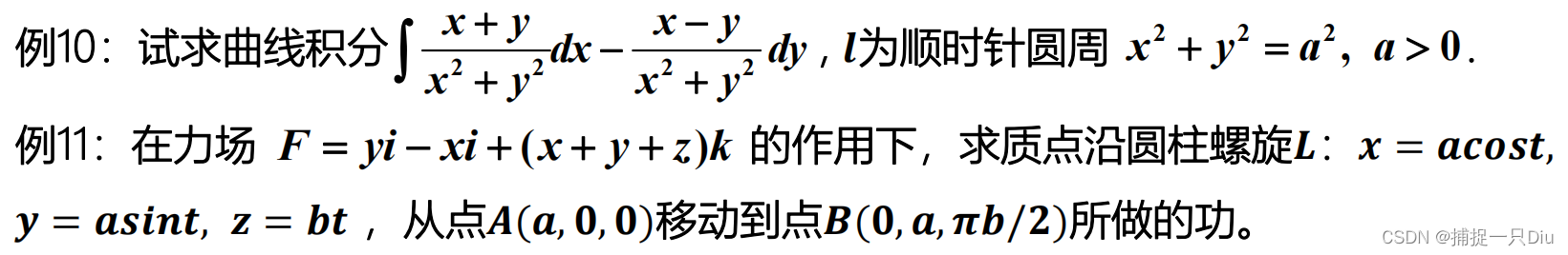
I10 = int(F*ds,t,2*pi,0)syms t
syms a b positive;
x = a*cos(t);
y = a*sin(t);
z = b*t;
F = [y,-x,(x+y+z)]; % 行向量
ds = [diff(x,t);diff(y,t);diff(z,t)]; % 列向量
I11 = int(F*ds,t,0,pi/2)

syms t x y z
x = 3*t;
y = 2*t;
z = t;
F = [x^3,3*z*y^2,-x^2*y];
ds = [diff(x,t);diff(y,t);diff(z,t)];
I12 = int(F*ds,t,1,0)

第一类曲面积分：

syms x y dx dy
z = sqrt(x^2+y^2);
ezsurf(z)
shading interp
hold on
ezmesh('1',70)
ezmesh('2',70)
axis([-2,2,-2,2,0,2.5])
alpha(0.5)  % 透明度
ds = simplify(sqrt(1+diff(z,x)^2+diff(z,y)^2)*dx*dy)
% ds = 2^(1/2)*dx*dy
% 再转换为极坐标计算
syms r theta;
I = sqrt(2)*int(int(r^3,r,1,2),theta,0,2*pi)

syms u v
syms a positive
x = u*cos(v); 
y = u*sin(v); 
z = v; 
f = x^2*y+z*y^2;
E = simplify(diff(x,u)^2+diff(y,u)^2+diff(z,u)^2);
F = simplify(diff(x,u)*diff(x,v)+diff(y,u)*diff(y,v)+diff(z,u)*diff(z,v));
G = simplify(diff(x,v)^2+diff(y,v)^2+diff(z,v)^2);
I = int(int(f*sqrt(E*G-F^2),u,0,a),v,0,2*pi)

第二类曲面积分： 

syms r theta
I = 2*int(int(r^3*sqrt(1-r^2)*sin(theta)*cos(theta),r,0,1),theta,0,pi/2)

七、级数求和与泰勒展式

syms n x m
s1 = symsum(1/n^2,n,1,inf)
s2 = symsum((-1)^(n+1)/n,1,inf) 
s3 = symsum(n*x^n,n,1,inf) 
s4 = symsum(n^2,1,100) 
J = limit(symsum(1/(m*(m+1)),m,1,n),n,inf) % symsum(1/n/(n+1),n,1,inf)

syms x
fh = exp(x);
ft = taylor(fh,x,0,'Order',10)
ezplot(fh)
hold on
ezplot(ft)

直接在命令行窗口输入taylortool即可打开。

八、符号方程求解

syms x
eqn1 = 1/(x+1) + 4*x/(x^2-4) == 1 + 2/(x-2);
sol1 = solve(eqn1,x)eqn2 = x-(x^3-4*x-7)^(1/3) == 1;
sol2 = solve(eqn2,x) eqn3 = x+x*exp(x)-10 == 0;
sol3 = solve(eqn3,x)  % 会警告
sol3 = vpasolve(eqn3,x)eqn4 = 2*sin(3*x-pi/4) == 1;
[solx,parameters,conditions] = solve(eqn4,x,'ReturnConditions',true)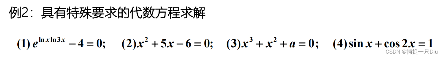

syms x
eqn1 = exp(log(x)*log(3*x))-4 == 0;
sol1 = solve(eqn1,x,'IgnoreAnalyticConstraints',true)
vpa(sol1)syms x positive
eqn2 = x^2 + 5*x - 6 == 0;
sol2 = solve(eqn2,x)
sol2 = solve(eqn2,x,'IgnoreProperties',true)
assume(x,'clear')syms x a
eqn3 = x^3 + x^2 + a == 0;
sol3 = solve(eqn3, x)
sol3 = solve(eqn3, x,'MaxDegree',3)syms x
eqn4 = sin(x) + cos(2*x) == 1;
sol4 = solve(eqn4,x)
sol4 = solve(eqn4,x,'PrincipalValue',true)

 

% syms x y positive
syms x y
eqn1 = [x^2 + y^2 - 5 == 0, 2*x^2 - 3*x*y - 2*y^2 == 0, x > 0, y > 0];
sol1 = solve(eqn1,[x,y],'ReturnConditions',true)
sol1.x
sol1.ysyms x y z
eqn2 = [sin(x)+y^2+log(z)-7 == 0, 3*x+2^y-z^3+1 == 0, x+y+z == 5];
sol2 = solve(eqn2,[x,y,z]); %vpasolve(eqn2,[x,y,z])
sol2.x
sol2.y
sol2.z
sol2 = vpasolve(eqn2,[x,y,z])

syms x y z u v
L = x^2+y^2+z^2+u*(x^2+y^2-z)+v*(x+y+z-1);
Lx = diff(L,x); 
Ly = diff(L,y); 
Lz = diff(L,z); 
Lu = diff(L,u); 
Lv = diff(L,v);
eqns = [Lx == 0, Ly == 0, Lz == 0, Lu == 0, Lv == 0];
sol = solve(eqns,[x,y,z,u,v])
sol.x
sol.y
sol.u
sol.v
for i = 1:4Lval(i) = vpa(subs(subs(subs(subs(subs(L,x,sol.x(i)),y,sol.y(i)),z,sol.z(i)),u,sol.u(i)),v,sol.v(i)),5);
end
Lval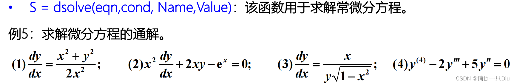

syms x y(x)
eqn2 = x^2*diff(y,x)+2*x*y-exp(x) == 0;
S2 = dsolve(eqn2)eqn4 = diff(y,x,4) - 2*diff(y,x,3) + 5*diff(y,x,2) == 0;
S4 = dsolve(eqn4)

syms x y(x) a b
eqn1 = diff(y,x) == 2*x*y^2;
cond1 = y(0) == 1;
ySol(x) = dsolve(eqn1,cond1)eqn2 = diff(y,x) == x^2/(1+y^2);
cond2 = y(2) == 1;
ySol2(x) = dsolve(eqn2,cond2)eqn4 = diff(y,x,2) == a^2*y;
Dy = diff(y,x);
cond4 = [y(0) == 1,Dy(pi/a) == 0];
ySol4(x) = dsolve(eqn4,cond4)
S4 = subs(ySol4,a,1);
ezplot(S4)eqn5 = diff(y,x)^2+y^2 == 1;
cond5 = y(0) == 0;
ySol5(x) = dsolve(eqn5,cond5)

syms x y(x)
eqn = diff(y,x) == -2*y/x + 4*x;
cond = y(1) == 2;
S = dsolve(eqn,cond)fh = @(x,y)-2*y./x + 4*x;
[t,y] = ode45(fh,[1,5],2);
subplot(1,2,1)
ezplot(S,[1,5])
hold on 
plot(t,y,'r-.')
Sy = subs(S,x,t);
err = abs(Sy - y);
subplot(1,2,2)
plot(t,err,'r*')

 

syms t f(t) g(t)
eqns = [diff(f,t) == 3*f+4*g, diff(g,t) == -4*f+3*g];
cond = [f(0) == 1, g(0) == 2];
[f,g] = dsolve(eqns,cond)
ezplot(f,[0,5])
hold on; 
ezplot(g,[0,5]) 
grid on
legend('f =cos(4*t)*exp(3*t) + 2*sin(4*t)*exp(3*t)','g =2*cos(4*t)*exp(3*t) - sin(4*t)*exp(3*t)')
title('微分方程组的解图像')

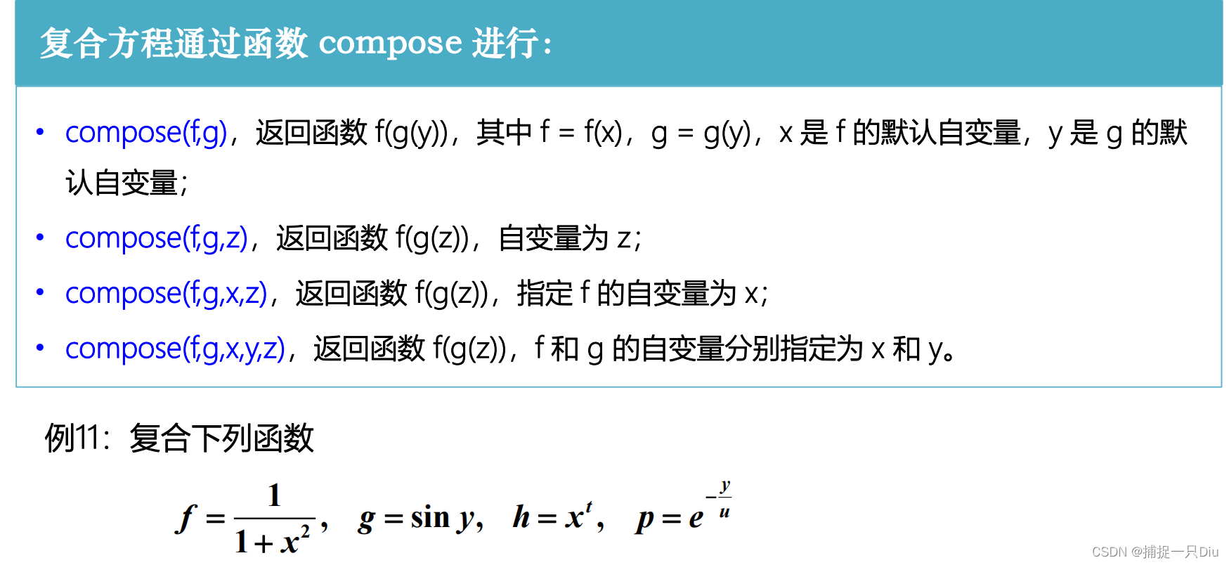
syms x y z t u
f = 1/(1 + x^2);
g = sin(y);
h = x^t;
p = exp(-y/u);
a = compose(f,g) % 默认自变量
b = compose(f,g,t) % 指定自变量为t
c = compose(h,g,x,z) % 指定h的自变量为x，且复合之后指定变量为z
e = compose(h,p,x,y,z) % 指定h自变量为x，p自变量为y，且复合之后指定变量为z
f = compose(h,p,t,u,z) % 指定h自变量为t，p自变量为u，且复合之后指定变量为z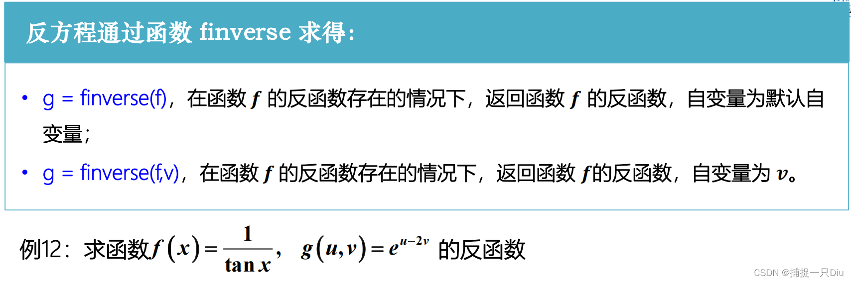

syms x u v
fh1 = 1/tan(x);
fh2 = exp(u-2*v);
ffh1 = finverse(fh1)
ffh2 = finverse(fh2,u)
ffh3 = finverse(fh2,v)

这篇关于MATLAB：符号运算的文章就介绍到这儿，希望我们推荐的文章对编程师们有所帮助！

---