本文主要是介绍共享单车线性回归分析,希望对大家解决编程问题提供一定的参考价值,需要的开发者们随着小编来一起学习吧!
给出共享单车的相关业务数据,建立kmeans模型,不同维度分群结果进行分析
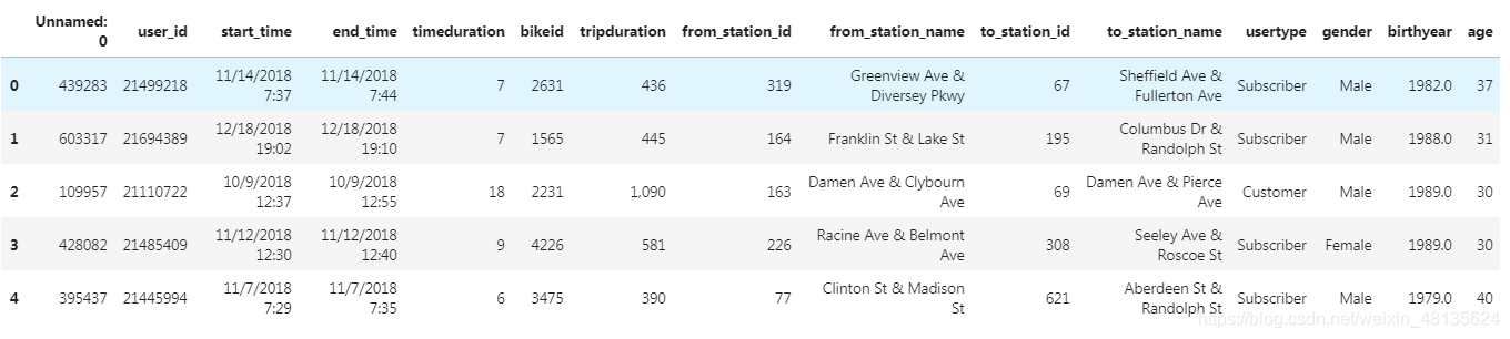
| column | definition |
|---|---|
| user_id | 用户编码 |
| start_time | 开始时间 |
| end_time | 结束时间 |
| timeduration | 骑行时长 |
| bikeid | 自行车编码 |
| tripduration | 骑行距离 |
| from_station_id | 开始站编码 |
| from_station_name | 开始站名字 |
| to_station_id | 结束站编码 |
| to_station_name | 结束站名字 |
| usertype | 用户种类 |
| gender | 性别 |
| birthyear | 出生年份 |
| age | 年龄 |
import pandas as pd
mobike=pd.read_csv("mobike.csv")
mobike.head()   #查看数据内容
mobike.info()   #查看数据类型,观察是否有缺失值<class 'pandas.core.frame.DataFrame'>
RangeIndex: 6427 entries, 0 to 6426
Data columns (total 15 columns):#   Column             Non-Null Count  Dtype
---  ------             --------------  -----  0   Unnamed: 0         6427 non-null   int64  1   user_id            6427 non-null   int64  2   start_time         6427 non-null   object 3   end_time           6427 non-null   object 4   timeduration       6427 non-null   int64  5   bikeid             6427 non-null   int64  6   tripduration       6427 non-null   object 7   from_station_id    6427 non-null   int64  8   from_station_name  6427 non-null   object 9   to_station_id      6427 non-null   int64  10  to_station_name    6427 non-null   object 11  usertype           6427 non-null   object 12  gender             5938 non-null   object 13  birthyear          5956 non-null   float6414  age                6427 non-null   object
dtypes: float64(1), int64(6), object(8)
memory usage: 753.3+ KBmobike.describe()  #结果的索引将包括计数,平均值,标准差,最小值,最大值以及较低的百分位数和50。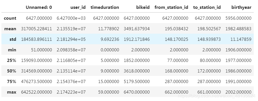
单变量分析
#删除无实际意义的索引行,inplace=True是直接在原始数据中保存排序之后的结果
mobike.drop("Unnamed: 0",inplace=True,axis=1)#类别型变量转换成数字型
#mobike['age'],对于age这个列做修改后的存储列
mobike['age']=mobike.age.str.replace('\'','').replace(' ','0').astype(int)
mobike.info()#此时的age变成int32类型<class 'pandas.core.frame.DataFrame'>
RangeIndex: 6427 entries, 0 to 6426
Data columns (total 14 columns):#   Column             Non-Null Count  Dtype
---  ------             --------------  -----  0   user_id            6427 non-null   int64  1   start_time         6427 non-null   object 2   end_time           6427 non-null   object 3   timeduration       6427 non-null   int64  4   bikeid             6427 non-null   int64  5   tripduration       6427 non-null   object 6   from_station_id    6427 non-null   int64  7   from_station_name  6427 non-null   object 8   to_station_id      6427 non-null   int64  9   to_station_name    6427 non-null   object 10  usertype           6427 non-null   object 11  gender             5938 non-null   object 12  birthyear          5956 non-null   float6413  age                6427 non-null   int32
dtypes: float64(1), int32(1), int64(5), object(7)
memory usage: 678.0+ KB#发现年龄最小是0最大是113,属于数据异常,进行数据清洗,这里保留用户年龄在18-70岁之间的群体
mobike=mobike[mobike['age']<=70]
mobike=mobike[mobike['age']>=18]
mobike.describe()user_id	    timeduration	bikeid	from_station_id	to_station_id	birthyear	age
count	5.939000e+03	5939.000000	5939.000000	5939.000000	5939.000000	5939.000000	5939.000000
mean	2.136120e+07	10.817309	3506.519448	196.996969	201.032665	1982.591177	36.408823
std	2.182745e+05	8.477247	1916.098846	148.159023	148.888064	10.924396	10.924396
min	2.098358e+07	0.000000	2.000000	2.000000	3.000000	1949.000000	18.000000
25%	2.117430e+07	5.000000	1853.500000	77.000000	81.000000	1977.000000	28.000000
50%	2.136393e+07	8.000000	3637.000000	172.000000	174.000000	1986.000000	33.000000
75%	2.154985e+07	14.000000	5207.500000	288.000000	288.000000	1991.000000	42.000000
max	2.174223e+07	59.000000	6470.000000	662.000000	661.000000	2001.000000	70.000000#将开始时间和结束时间转变为日期时间格式,object换成datetime64
mobike['start_time']=pd.to_datetime(mobike['start_time'])
mobike['end_time']=pd.to_datetime(mobike['end_time'])
mobike.info()<class 'pandas.core.frame.DataFrame'>
Int64Index: 5939 entries, 0 to 6426
Data columns (total 14 columns):#   Column             Non-Null Count  Dtype
---  ------             --------------  -----         0   user_id            5939 non-null   int64         1   start_time         5939 non-null   datetime64[ns]2   end_time           5939 non-null   datetime64[ns]3   timeduration       5939 non-null   int64         4   bikeid             5939 non-null   int64         5   tripduration       5939 non-null   object        6   from_station_id    5939 non-null   int64         7   from_station_name  5939 non-null   object        8   to_station_id      5939 non-null   int64         9   to_station_name    5939 non-null   object        10  usertype           5939 non-null   object        11  gender             5922 non-null   object        12  birthyear          5939 non-null   float64       13  age                5939 non-null   int32
dtypes: datetime64[ns](2), float64(1), int32(1), int64(5), object(5)
memory usage: 672.8+ KBmobike.drop(mobike.select_dtypes(['datetime64']),inplace=True,axis=1)
#inplace=True直接在原始数据中保存排序之后的结果
#axis 列索引,表名不同列,纵向索引,叫columns,1轴,axis=1#把骑行事件中的逗号进行类型转换.(逗号替换掉)
mobike['tripduration'] = mobike['tripduration'].str.replace(',','').astype(int)mobike['tripduration']
0        436
1        445
2       1090
3        581
4        390...
6422     431
6423     918
6424    1165
6425     500
6426     483
Name: tripduration, Length: 5939, dtype: int32
mobike_ = mobike[['usertype','gender']]#把性别里面的缺失值用unkown代替作为填充.
mobike.gender.fillna('unkown',inplace=True)#用户渠道分类统计
mobike.groupby(["usertype"]).count() #Customer注册的,Subscriber没注册的.

pd.get_dummies(mobike_) #可以分别做哑变量转换,也可以放在一起.此时把这两列做一个哑变量矩阵#将类别性别转化成哑变量(gender)
# mobike["gender"]= pd.get_dummies(mobike.gender)
# mobike["gender"]
#将类别用户种类转化成哑变量(usertype)
# mobike["usertype"]= pd.get_dummies(mobike.usertype)
# mobike["usertype"]

mobike["gender"].value_counts()  #性别个数数据统计
Male      4623
Female    1299
unkown      17
Name: gender, dtype: int64#查看当前有多少列,列名分别时什么。
mobike.columns
Index(['user_id', 'timeduration', 'bikeid', 'tripduration', 'from_station_id','from_station_name', 'to_station_id', 'to_station_name', 'usertype','gender', 'birthyear', 'age'],dtype='object')#pd.concat实现数据合并 ,传入的第一个数据是预处理的数据。
mobike_one_hot=pd.concat([mobike,pd.get_dummies(mobike_)],axis=1)
mobike_one_hot.columns
Index(['user_id', 'timeduration', 'bikeid', 'tripduration', 'from_station_id','from_station_name', 'to_station_id', 'to_station_name', 'usertype','gender', 'birthyear', 'age', 'gender_Female', 'gender_Male','gender_unkown', 'usertype_Customer', 'usertype_Subscriber'],dtype='object')
mobike_one_hot
结果展示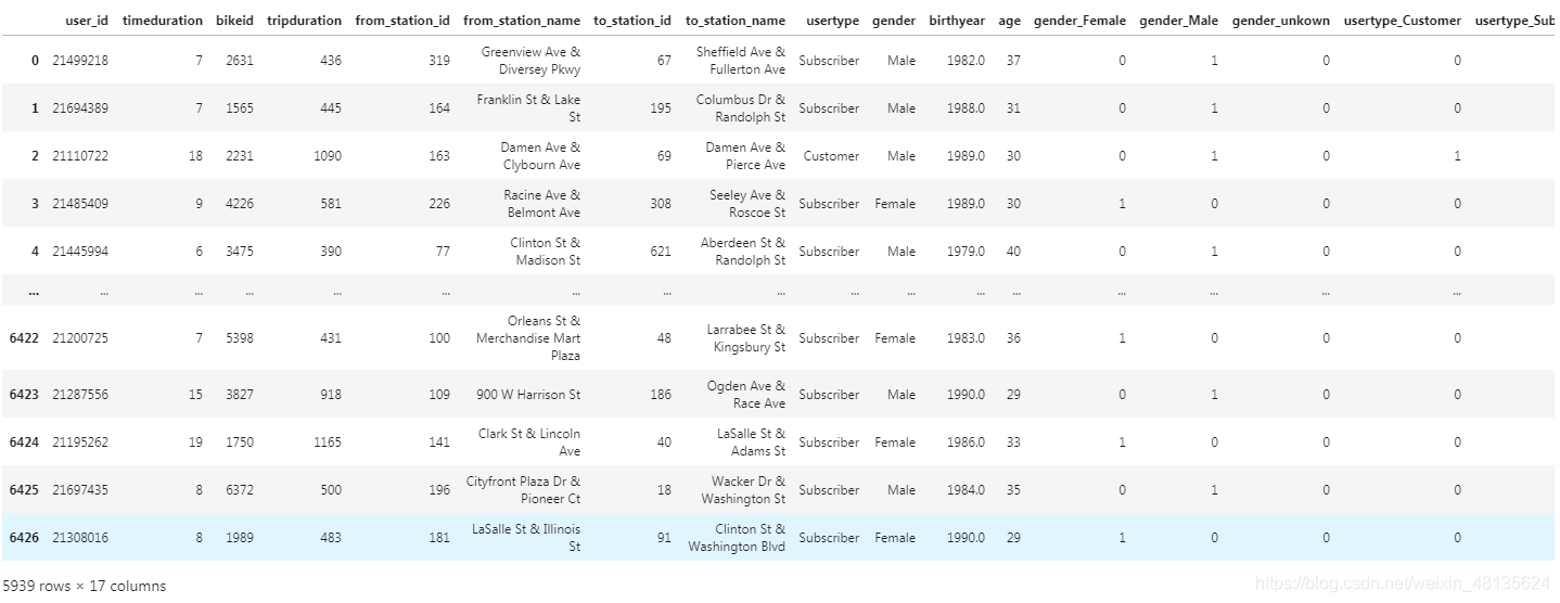
tripduration中的233732属于不正常的距离,需要进行数据清洗
mobike_= mobike_one_hot[['timeduration','tripduration', 'age','usertype_Customer', 'usertype_Subscriber', 'gender_Female','gender_Male', 'gender_unkown']]mobike_3=mobike_one_hot[["timeduration","tripduration","age","gender_Female","gender_Male","usertype_Customer","usertype_Subscriber"]]mobike_2= mobike_one_hot[['tripduration', 'age','usertype_Customer', 'usertype_Subscriber']]mobike.describe()user_id	timeduration	bikeid	tripduration	from_station_id	to_station_id	birthyear	age
count	5.939000e+03	5939.000000	5939.000000	5939.000000	5939.000000	5939.000000	5939.000000	5939.000000
mean	2.136120e+07	10.817309	3506.519448	793.080485	196.996969	201.032665	1982.591177	36.408823
std	2.182745e+05	8.477247	1916.098846	3334.075550	148.159023	148.888064	10.924396	10.924396
min	2.098358e+07	0.000000	2.000000	61.000000	2.000000	3.000000	1949.000000	18.000000
25%	2.117430e+07	5.000000	1853.500000	338.500000	77.000000	81.000000	1977.000000	28.000000
50%	2.136393e+07	8.000000	3637.000000	527.000000	172.000000	174.000000	1986.000000	33.000000
75%	2.154985e+07	14.000000	5207.500000	857.000000	288.000000	288.000000	1991.000000	42.000000
max	2.174223e+07	59.000000	6470.000000	233732.000000	662.000000	661.000000	2001.000000	70.000000#由上表可知tripduration属于不正常的距离。所以把大于10000的统计之后,做删除处理。
mobike[mobike["tripduration"]>10000].count()user_id              15
timeduration         15
bikeid               15
tripduration         15
from_station_id      15
from_station_name    15
to_station_id        15
to_station_name      15
usertype             15
gender               15
birthyear            15
age                  15
dtype: int64mobike=mobike[mobike['tripduration']<10000]
mobike.describe()user_id	timeduration	bikeid	tripduration	from_station_id	to_station_id	birthyear	age
count	5.924000e+03	5924.000000	5924.000000	5924.000000	5924.000000	5924.000000	5924.000000	5924.000000
mean	2.136154e+07	10.739872	3506.339804	704.265361	197.110230	200.842674	1982.594531	36.405469
std	2.181799e+05	8.291724	1916.579026	664.976888	148.199333	148.559883	10.921172	10.921172
min	2.098358e+07	0.000000	2.000000	61.000000	2.000000	3.000000	1949.000000	18.000000
25%	2.117469e+07	5.000000	1853.000000	337.750000	77.000000	81.000000	1977.000000	28.000000
50%	2.136492e+07	8.000000	3635.500000	526.500000	173.000000	174.000000	1986.000000	33.000000
75%	2.155034e+07	14.000000	5207.250000	854.250000	288.250000	288.000000	1991.000000	42.000000
max	2.174223e+07	59.000000	6470.000000	9893.000000	662.000000	661.000000	2001.000000	70.000000
查看数据之间的相关度
#如何查看相关性 corr计算的是夹角的余弦值[-1,1].一般情况下骑得越久就越远,还是有相关性的。
mobike.corr() # 0.269336是有相关性的,0.2到0.3会有一个很明显的相关性,如果到0.3以上有明显的相关性;0.5以上有强相关性
#建模时分群tripduration和timeduration可以只用其中一个,因为用户特征比较明显;也可以两个都用。
选择七个变量mobike_3作为分群的维度,数据标准化后,进行聚类分析。
mobike_3=mobike_one_hot[["timeduration","tripduration","age","gender_Female","gender_Male","usertype_Customer","usertype_Subscriber"]]#Standardization标准化:将特征数据的分布调整成标准正太分布,也叫高斯分布,也就是使得数据的均值维0,方差为1.
#数据标准化,使用sklearn中预处理的scale
#duration=mobike_3[['tripduration','timeduration']]
#from sklearn.preprocessing import scale
#x1=pd.DataFrame(scale(duration))
#x1
mobike_3["tripduration"]=(mobike_3["tripduration"]-mobike_3["tripduration"].mean())/mobike_3["tripduration"].std()
#(收入-收入均值)/收入标准差
mobike_3["timeduration"]=(mobike_3["timeduration"]-mobike_3["timeduration"].mean())/mobike_3["timeduration"].std()#数据进行标准化后的结果,先尝试分为3类
model=KMeans(n_clusters=3,random_state=10)  #n_clusters=3,分成三类,random_state自动生成随机数固定。
model.fit(mobike_3)
#提取标签,查看分类结果
mobike_3['cluster']=model.labels_   #把聚类的结果放成一列排在下面表中
mobike_3.groupby("cluster").age.count()显示结果
cluster
0    2797
1    1144
2    1998
Name: age, dtype: int64#使用groupby函数,评估各个变量维度的分群效果
mobike_3.groupby(['cluster'])['age'].describe()    count	   mean	        std	     min	 25%	 50%	75%	    max
cluster
0	2797.0	27.701108	3.019970	18.0	26.0	28.0	30.0	32.0
1	1144.0	55.107517	5.712397	47.0	50.0	55.0	59.0	70.0
2	1998.0	37.892392	3.836275	33.0	35.0	37.0	41.0	46.0结论:从mobike_3可以看出通过年龄分成三组,18岁-32岁;33岁-46岁;47岁-70岁.
结论:从mobike_3可以看出通过年龄分成三组,18岁-32岁;33岁-46岁;47岁-70岁.
模型评估与优化
from sklearn import metrics#调用sklearn的metrics库
from sklearn.preprocessing import scale
#x_cluster=model.fit_predict(mobike_3)#个体与群的距离,不能用这句来执行,因为包含了cluster.所以提取所需要的值.
x_cluster = model.fit_predict(mobike_3[['timeduration','tripduration', 'age','usertype_Customer', 'usertype_Subscriber', 'gender_Female','gender_Male']])score=metrics.silhouette_score(mobike_3[['timeduration','tripduration', 'age','usertype_Customer', 'usertype_Subscriber', 'gender_Female','gender_Male']],x_cluster)#评分越高,个体与群越近;评分越低,个体与群越远
#print(score)
#0.5399278008634186
centers=pd.DataFrame(model.cluster_centers_,columns=["timeduration","tripduration","age","gender_Female","gender_Male","usertype_Customer","usertype_Subscriber"])
centers| timeduration | tripduration | age | gender_Female | gender_Male | usertype_Customer | usertype_Subscriber | |
|---|---|---|---|---|---|---|---|
| 0 | -0.020076 | 0.006295 | 27.701108 | 0.042188 | 0.957812 | 0.258849 | 0.738649 |
| 1 | 0.048773 | 0.018423 | 55.107517 | 0.026224 | 0.973776 | 0.180070 | 0.817308 |
| 2 | 0.000178 | -0.019362 | 37.892392 | 0.030531 | 0.969469 | 0.184685 | 0.811812 |
选择四个变量mobike_2作为分群的维度,数据标准化后,进行聚类分析。
mobike_2=mobike_one_hot[["tripduration","age","usertype_Customer","usertype_Subscriber"]]
mobike_2["tripduration"]=(mobike_2["tripduration"]-mobike_2["tripduration"].mean())/mobike_2["tripduration"].std()
mobike_2["age"]=(mobike_2["age"]-mobike_2["age"].mean())/mobike_2["age"].std()#数据进行标准化后的结果,先尝试分为3类
model=KMeans(n_clusters=3,random_state=10)  #n_clusters=3,分成三类,random_state自动生成随机数固定。
model.fit(mobike_2)
#提取标签,查看分类结果
mobike_2['cluster']=model.labels_   #把聚类的结果放成一列排在下面表中
mobike_2.groupby("cluster").count()显示结果tripduration	age	usertype_Customer	usertype_Subscriber
cluster
0	   4375	        4375	 4375	             4375
1	   1563	        1563	 1563	             1563
2	    1	         1	      1	                   1mobike_2["cluster"].count()
显示结果
5939
模型评估与优化
x_cluster = model.fit_predict(mobike_2[["tripduration","age","usertype_Customer","usertype_Subscriber"]])
score=metrics.silhouette_score(mobike_2[["tripduration","age","usertype_Customer","usertype_Subscriber"]],x_cluster)#评分越高,个体与群越近;评分越低,个体与群越远
print(score)
0.6183295392287478centers=pd.DataFrame(model.cluster_centers_,columns=["tripduration","age","usertype_Customer","usertype_Subscriber"])
centers
| tripduration | age | usertype_Customer | usertype_Subscriber | |
|---|---|---|---|---|
| 0 | 0.005522 | 1.434627 | 0.027511 | 0.972489 |
| 1 | -0.017942 | -0.512187 | 0.037943 | 0.962057 |
| 2 | 69.866119 | -1.502035 | 0.000000 | 1.000000 |
这篇关于共享单车线性回归分析的文章就介绍到这儿,希望我们推荐的文章对编程师们有所帮助!


