2、 Scheduler介绍代码解析 [代码级手把手解diffusers库]

本文主要是介绍2、 Scheduler介绍代码解析 [代码级手把手解diffusers库]，希望对大家解决编程问题提供一定的参考价值，需要的开发者们随着小编来一起学习吧！

- Scheduler简介
- 分类
- - 老式 ODE 求解器（Old-School ODE solvers）
  - 初始采样器（Ancestral samplers）
  - Karras噪声调度计划
  - DDIM和PLMS
  - DPM、DPM adaptive、DPM2和 DPM++
  - UniPC
  - k-diffusion
- 1.DDPM
- 2.DDIM
- 3.Euler
- 4.DPM系列
- 5. Ancestral
- 6. Karras
- 7. SDE

Scheduler简介

Diffusion Pipeline 本质上是彼此部分独立的模型和调度器的集合。Diffusion中最重要的我觉得一定是Scheduler，因为它这里面包含了扩散模型的基本原理，通过对代码的分析我们可以对论文中的公式有着更好的理解，同时diffusers也在DDPM的基础上优化了许多不同的scheduler版本，加深对这些scheduler的理解也可以帮助我们在实际选择scheduler时有更好的理论支持：

在这里插入图片描述
Scheduler直观上理解的话它就是一个采样器，循环多个step把噪声图像逐渐还原为原始图像(xt -> x0)。根据采样方式不同，scheduler也有许多版本，包括DDPM，DDIM，DPM++ 2M Karras等，通常决定了去噪速度和去噪质量。注意：看下面内容前最好对扩散模型的原理有一定了解，可参考论文DDPM。

StableDiffusionPipeline中默认的调度器是PNDMScheduler：

from huggingface_hub import login
from diffusers import DiffusionPipeline
import torch
pipeline = DiffusionPipeline.from_pretrained("runwayml/stable-diffusion-v1-5", torch_dtype=torch.float16, use_safetensors=True)
pipeline.to("cuda")
print(pipeline.scheduler)

输出如下：

PNDMScheduler {"_class_name": "PNDMScheduler","_diffusers_version": "0.21.4","beta_end": 0.012,"beta_schedule": "scaled_linear","beta_start": 0.00085,"clip_sample": false,"num_train_timesteps": 1000,"set_alpha_to_one": false,"skip_prk_steps": true,"steps_offset": 1,"timestep_spacing": "leading","trained_betas": null
}

对于不同的Pipeline，我们可以用pipeline.scheduler.compatibles，查看它都有哪些适配的调度器，如StableDiffusionPipeline：

[diffusers.utils.dummy_torch_and_torchsde_objects.DPMSolverSDEScheduler,diffusers.schedulers.scheduling_euler_discrete.EulerDiscreteScheduler,diffusers.schedulers.scheduling_lms_discrete.LMSDiscreteScheduler,diffusers.schedulers.scheduling_ddim.DDIMScheduler,diffusers.schedulers.scheduling_ddpm.DDPMScheduler,diffusers.schedulers.scheduling_heun_discrete.HeunDiscreteScheduler,diffusers.schedulers.scheduling_dpmsolver_multistep.DPMSolverMultistepScheduler,diffusers.schedulers.scheduling_deis_multistep.DEISMultistepScheduler,diffusers.schedulers.scheduling_pndm.PNDMScheduler,diffusers.schedulers.scheduling_euler_ancestral_discrete.EulerAncestralDiscreteScheduler,diffusers.schedulers.scheduling_unipc_multistep.UniPCMultistepScheduler,diffusers.schedulers.scheduling_k_dpm_2_discrete.KDPM2DiscreteScheduler,diffusers.schedulers.scheduling_dpmsolver_singlestep.DPMSolverSinglestepScheduler,diffusers.schedulers.scheduling_k_dpm_2_ancestral_discrete.KDPM2AncestralDiscreteScheduler]

使用pipeline.scheduler.config，我们可用轻松的获得当前pipe调度器的配置参数，这些参数都是Diffusion迭代去噪过程的控制参数（具体原理参考论文），如StableDiffusionPipeline：

FrozenDict([('num_train_timesteps', 1000),('beta_start', 0.00085),('beta_end', 0.012),('beta_schedule', 'scaled_linear'),('trained_betas', None),('skip_prk_steps', True),('set_alpha_to_one', False),('prediction_type', 'epsilon'),('timestep_spacing', 'leading'),('steps_offset', 1),('_use_default_values', ['timestep_spacing', 'prediction_type']),('_class_name', 'PNDMScheduler'),('_diffusers_version', '0.21.4'),('clip_sample', False)])

有了这些参数，我们可以轻松的更换不同的Scheduler，具体选择哪个还得多尝试：

from diffusers import DDIMScheduler
pipeline.scheduler = DDIMScheduler.from_config(pipeline.scheduler.config)from diffusers import LMSDiscreteScheduler
pipeline.scheduler = LMSDiscreteScheduler.from_config(pipeline.scheduler.config)from diffusers import EulerDiscreteScheduler
pipeline.scheduler = EulerDiscreteScheduler.from_config(pipeline.scheduler.config)from diffusers import EulerAncestralDiscreteScheduler
pipeline.scheduler = EulerAncestralDiscreteScheduler.from_config(pipeline.scheduler.config)from diffusers import DPMSolverMultistepScheduler
pipeline.scheduler = DPMSolverMultistepScheduler.from_config(pipeline.scheduler.config)

1.DDPM

接下来我们先以最基础的DDPM为例，分析diffusers库里的对应代码。代码在

diffusers/src/diffusers/schedulers/scheduling_ddpm.py中，以下是核心部分step函数的代码。

step函数完成的操作就是，在去噪过程中：

输入：UNet预测的pred_noise(model_output)、当前timestep(timestep)、当前的latents(sample)。
输出：该timestep去噪后的latents。

    def step(self,model_output: torch.FloatTensor,timestep: int,sample: torch.FloatTensor,generator=None,return_dict: bool = True,) -> Union[DDPMSchedulerOutput, Tuple]:"""Predict the sample from the previous timestep by reversing the SDE. This function propagates the diffusionprocess from the learned model outputs (most often the predicted noise).Args:model_output (`torch.FloatTensor`):The direct output from learned diffusion model.timestep (`float`):The current discrete timestep in the diffusion chain.sample (`torch.FloatTensor`):A current instance of a sample created by the diffusion process.generator (`torch.Generator`, *optional*):A random number generator.return_dict (`bool`, *optional*, defaults to `True`):Whether or not to return a [`~schedulers.scheduling_ddpm.DDPMSchedulerOutput`] or `tuple`.Returns:[`~schedulers.scheduling_ddpm.DDPMSchedulerOutput`] or `tuple`:If return_dict is `True`, [`~schedulers.scheduling_ddpm.DDPMSchedulerOutput`] is returned, otherwise atuple is returned where the first element is the sample tensor."""t = timestepprev_t = self.previous_timestep(t)if model_output.shape[1] == sample.shape[1] * 2 and self.variance_type in ["learned", "learned_range"]:model_output, predicted_variance = torch.split(model_output, sample.shape[1], dim=1)else:predicted_variance = None# 1. compute alphas_t, betas_talpha_prod_t = self.alphas_cumprod[t]alpha_prod_t_prev = self.alphas_cumprod[prev_t] if prev_t >= 0 else self.onebeta_prod_t = 1 - alpha_prod_tbeta_prod_t_prev = 1 - alpha_prod_t_prevcurrent_alpha_t = alpha_prod_t / alpha_prod_t_prevcurrent_beta_t = 1 - current_alpha_t# 2. compute predicted original sample from predicted noise also called# "predicted x_0" of formula (15) from https://arxiv.org/pdf/2006.11239.pdfif self.config.prediction_type == "epsilon":pred_original_sample = (sample - beta_prod_t ** (0.5) * model_output) / alpha_prod_t ** (0.5)elif self.config.prediction_type == "sample":pred_original_sample = model_outputelif self.config.prediction_type == "v_prediction":pred_original_sample = (alpha_prod_t**0.5) * sample - (beta_prod_t**0.5) * model_outputelse:raise ValueError(f"prediction_type given as {self.config.prediction_type} must be one of `epsilon`, `sample` or"" `v_prediction`  for the DDPMScheduler.")# 3. Clip or threshold "predicted x_0"if self.config.thresholding:pred_original_sample = self._threshold_sample(pred_original_sample)elif self.config.clip_sample:pred_original_sample = pred_original_sample.clamp(-self.config.clip_sample_range, self.config.clip_sample_range)# 4. Compute coefficients for pred_original_sample x_0 and current sample x_t# See formula (7) from https://arxiv.org/pdf/2006.11239.pdfpred_original_sample_coeff = (alpha_prod_t_prev ** (0.5) * current_beta_t) / beta_prod_tcurrent_sample_coeff = current_alpha_t ** (0.5) * beta_prod_t_prev / beta_prod_t# 5. Compute predicted previous sample µ_t# See formula (7) from https://arxiv.org/pdf/2006.11239.pdfpred_prev_sample = pred_original_sample_coeff * pred_original_sample + current_sample_coeff * sample# 6. Add noisevariance = 0if t > 0:device = model_output.devicevariance_noise = randn_tensor(model_output.shape, generator=generator, device=device, dtype=model_output.dtype)if self.variance_type == "fixed_small_log":variance = self._get_variance(t, predicted_variance=predicted_variance) * variance_noiseelif self.variance_type == "learned_range":variance = self._get_variance(t, predicted_variance=predicted_variance)variance = torch.exp(0.5 * variance) * variance_noiseelse:variance = (self._get_variance(t, predicted_variance=predicted_variance) ** 0.5) * variance_noisepred_prev_sample = pred_prev_sample + varianceif not return_dict:return (pred_prev_sample,)return DDPMSchedulerOutput(prev_sample=pred_prev_sample, pred_original_sample=pred_original_sample)

大家从注释可以看出个大概，但是代码里面可能包含了一些额外的if判断导致不是很清楚，所以我把其中最关键的几句骨架提取出来。

alpha_prod_t = self.alphas_cumprod[t]
alpha_prod_t_prev = self.alphas_cumprod[prev_t] if prev_t >= 0 else self.one
beta_prod_t = 1 - alpha_prod_t
beta_prod_t_prev = 1 - alpha_prod_t_prev
current_alpha_t = alpha_prod_t / alpha_prod_t_prev
current_beta_t = 1 - current_alpha_t

以上代码作用是计算当前step的alpha和beta的对应参数，以上变量分别对应了论文中的

在这里插入图片描述

pred_original_sample = (sample - beta_prod_t ** (0.5) * model_output) / alpha_prod_t ** (0.5)

以上代码根据模型的预测噪声推出原始图像x_{0}，也就是对应论文中公式（15），其中sample就是 $x_{t}$ ，代表当前step的加噪图像，model_output代表模型的预测噪声 $\epsilon$ 。
在这里插入图片描述

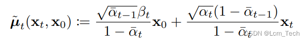
pred_original_sample_coeff = (alpha_prod_t_prev ** (0.5) * current_beta_t) / beta_prod_t
current_sample_coeff = current_alpha_t ** (0.5) * beta_prod_t_prev / beta_prod_tpred_prev_sample = pred_original_sample_coeff * pred_original_sample + current_sample_coeff * sample

以上代码计算了 $x_{0}$ 和 $x_{t}$ 的系数，对应公式（7）， $x_{0}$ 代表上一步计算的原始图像， $x_{t}$ 代表当前step的加噪图像，\mu _{t}代表的是分布的均值，对应着代码中的pred_prev_sample。

在这里插入图片描述

pred_prev_sample = pred_prev_sample + variance

最后则是在均值上加上噪声variance。

所以总体而言，整个流程满足公式（6），相当于是在基于 $x_{0}$ 和 $x_{t}$ 基础上 $x_{t-1}$ 的条件概率，而同时也是求一个分布，其中方差（即噪声）完全由step决定，而均值则由初始图像 $x_{0}$ 和当前噪声图像 $x_{t}$ 决定， $x_{0}$ 又通过模型预测得到噪声 $\epsilon$ 计算得到。

在这里插入图片描述

2.DDIM

DDIM就是针对上述DDPM的缺点，对DDPM进行改进的，来提高推理时间，去除了马尔可夫条件的限制，重新推导出逆向扩散方程，在代码scheduling_ddim.py中我们也可以看到对应的修改：
在这里插入图片描述

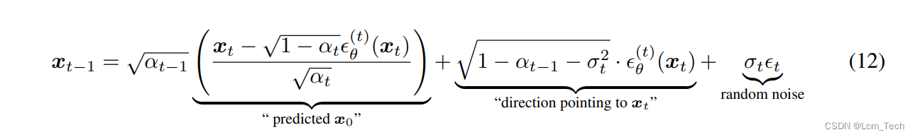
std_dev_t = eta * variance ** (0.5)
pred_sample_direction = (1 - alpha_prod_t_prev - std_dev_t**2) ** (0.5) * pred_epsilon
prev_sample = alpha_prod_t_prev ** (0.5) * pred_original_sample + pred_sample_directionprev_sample = prev_sample + variance

这样我们就可以每次迭代中跨多个step，从而减少推理迭代次数和时间。

3.Euler

当然除了基于DDIM之外还有很多不同原理的采样器，比如Euler，它是基于ODE的比较基础的采样器，以下是Euler在diffusers库scheduling_euler_discrete.py中的核心代码：

pred_original_sample = sample - sigma_hat * model_outputderivative = (sample - pred_original_sample) / sigma_hat
dt = self.sigmas[self.step_index + 1] - sigma_hat
prev_sample = sample + derivative * dt

从代码中可以看出大概的流程：通过对应step的噪声程度预测初始图像，然后通过微分求得对应的梯度方向，然后再向该方向迈进一定步长。

4.DPM系列

DPM++则会自适应调整步长，DPM2额外考虑了二阶动量，使得结果更准确，但速度更慢。

5. Ancestral

如果加了a，则表示每次采样后会加噪声，这样可能会导致最后不收敛，但随机性会更强。

6. Karras

如果加了Karras，则代表使用了特定的Karras噪声step表。

7. SDE

如果加了SDE，则代表使用了Score-based SDE方法，使采样过程更加稳定。

这篇关于2、 Scheduler介绍代码解析 [代码级手把手解diffusers库]的文章就介绍到这儿，希望我们推荐的文章对编程师们有所帮助！

2、 Scheduler介绍代码解析 [代码级手把手解diffusers库]

Scheduler简介

分类

老式 ODE 求解器（Old-School ODE solvers）

初始采样器（Ancestral samplers）

Karras噪声调度计划

DDIM和PLMS

DPM、DPM adaptive、DPM2和 DPM++

UniPC

k-diffusion

1.DDPM

2.DDIM

3.Euler

4.DPM系列

5. Ancestral

6. Karras

7. SDE

相关文章

Python使用Tenacity一行代码实现自动重试详解

深度解析Spring Security 中的 SecurityFilterChain核心功能

MySQL常用字符串函数示例和场景介绍

全面解析Golang 中的 Gorilla CORS 中间件正确用法

Mysql中设计数据表的过程解析

深度解析Nginx日志分析与499状态码问题解决

MySQL CTE (Common Table Expressions)示例全解析

Spring Boot 3.x 中 WebClient 示例详解析

在MySQL中实现冷热数据分离的方法及使用场景底层原理解析

C#解析JSON数据全攻略指南

2、 Scheduler介绍 代码解析 [代码级手把手解diffusers库]

Scheduler简介

分类

老式 ODE 求解器（Old-School ODE solvers）

初始采样器（Ancestral samplers）

Karras噪声调度计划

DDIM和PLMS

DPM、DPM adaptive、DPM2和 DPM++

UniPC

k-diffusion

1.DDPM

2.DDIM

3.Euler

4.DPM系列

5. Ancestral

6. Karras

7. SDE

相关文章

2、 Scheduler介绍代码解析 [代码级手把手解diffusers库]