深度学习第P8周：YOLOv5-C3模块实现

🏡 我的环境：
语言环境：Python3.8
编译器：Jupyter Lab
数据集：天气识别数据集
深度学习环境：Pytorch
torch1.12.1+cu113
torchvision0.13.1+cu113

一、 前期准备

1. 设置GPU

如果设备上支持GPU就使用GPU,否则使用CPU

import torch
import torch.nn as nn
import torchvision.transforms as transforms
import torchvision
from torchvision import transforms, datasets
import os,PIL,pathlib,warningswarnings.filterwarnings("ignore")             #忽略警告信息device = torch.device("cuda" if torch.cuda.is_available() else "cpu")
device

device(type='cuda')

2. 导入数据

import os,PIL,random,pathlibdata_dir = './data/8-data/'
data_dir = pathlib.Path(data_dir)data_paths  = list(data_dir.glob('*'))
classeNames = [str(path).split("\\")[2] for path in data_paths]
classeNames

['cloudy', 'rain', 'shine', 'sunrise']

# 关于transforms.Compose的更多介绍可以参考：https://blog.csdn.net/qq_38251616/article/details/124878863
train_transforms = transforms.Compose([transforms.Resize([224, 224]),  # 将输入图片resize成统一尺寸# transforms.RandomHorizontalFlip(), # 随机水平翻转transforms.ToTensor(),          # 将PIL Image或numpy.ndarray转换为tensor，并归一化到[0,1]之间transforms.Normalize(           # 标准化处理-->转换为标准正太分布（高斯分布），使模型更容易收敛mean=[0.485, 0.456, 0.406],std=[0.229, 0.224, 0.225])  # 其中 mean=[0.485,0.456,0.406]与std=[0.229,0.224,0.225] 从数据集中随机抽样计算得到的。
])test_transform = transforms.Compose([transforms.Resize([224, 224]),  # 将输入图片resize成统一尺寸transforms.ToTensor(),          # 将PIL Image或numpy.ndarray转换为tensor，并归一化到[0,1]之间transforms.Normalize(           # 标准化处理-->转换为标准正太分布（高斯分布），使模型更容易收敛mean=[0.485, 0.456, 0.406],std=[0.229, 0.224, 0.225])  # 其中 mean=[0.485,0.456,0.406]与std=[0.229,0.224,0.225] 从数据集中随机抽样计算得到的。
])total_data = datasets.ImageFolder("./data/8-data/",transform=train_transforms)
total_data

Dataset ImageFolderNumber of datapoints: 1125Root location: ./data/8-data/StandardTransform
Transform: Compose(Resize(size=[224, 224], interpolation=bilinear, max_size=None, antialias=None)ToTensor()Normalize(mean=[0.485, 0.456, 0.406], std=[0.229, 0.224, 0.225]))

total_data.class_to_idx

{'cloudy': 0, 'rain': 1, 'shine': 2, 'sunrise': 3}

3. 划分数据集

train_size = int(0.8 * len(total_data))
test_size  = len(total_data) - train_size
train_dataset, test_dataset = torch.utils.data.random_split(total_data, [train_size, test_size])
train_dataset, test_dataset

(<torch.utils.data.dataset.Subset at 0xf4a3c50>,<torch.utils.data.dataset.Subset at 0xf4a3e80>)

batch_size = 4train_dl = torch.utils.data.DataLoader(train_dataset,batch_size=batch_size,shuffle=True,num_workers=1)
test_dl = torch.utils.data.DataLoader(test_dataset,batch_size=batch_size,shuffle=True,num_workers=1)

for X, y in test_dl:print("Shape of X [N, C, H, W]: ", X.shape)print("Shape of y: ", y.shape, y.dtype)break

Shape of X [N, C, H, W]:  torch.Size([4, 3, 224, 224])
Shape of y:  torch.Size([4]) torch.int64

二、搭建包含C3模块的模型

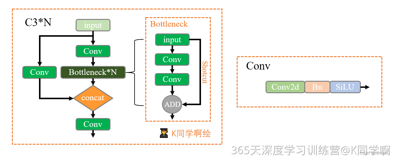
📌K同学啊提示：是否可以尝试通过增加/调整C3模块与Conv模块来提高准确率？
image.png

1. 搭建模型

import torch.nn.functional as Fdef autopad(k, p=None):  # kernel, padding# Pad to 'same'if p is None:p = k // 2 if isinstance(k, int) else [x // 2 for x in k]  # auto-padreturn pclass Conv(nn.Module):# Standard convolutiondef __init__(self, c1, c2, k=1, s=1, p=None, g=1, act=True):  # ch_in, ch_out, kernel, stride, padding, groupssuper().__init__()self.conv = nn.Conv2d(c1, c2, k, s, autopad(k, p), groups=g, bias=False)self.bn = nn.BatchNorm2d(c2)self.act = nn.SiLU() if act is True else (act if isinstance(act, nn.Module) else nn.Identity())def forward(self, x):return self.act(self.bn(self.conv(x)))def forward_fuse(self, x):return self.act(self.conv(x))class Bottleneck(nn.Module):# Standard bottleneckdef __init__(self, c1, c2, shortcut=True, g=1, e=0.5):  # ch_in, ch_out, shortcut, groups, expansionsuper().__init__()c_ = int(c2 * e)  # hidden channelsself.cv1 = Conv(c1, c_, 1, 1)self.cv2 = Conv(c_, c2, 3, 1, g=g)self.add = shortcut and c1 == c2def forward(self, x):return x + self.cv2(self.cv1(x)) if self.add else self.cv2(self.cv1(x))class C3(nn.Module):# CSP Bottleneck with 3 convolutionsdef __init__(self, c1, c2, n=1, shortcut=True, g=1, e=0.5):  # ch_in, ch_out, number, shortcut, groups, expansionsuper().__init__()c_ = int(c2 * e)  # hidden channelsself.cv1 = Conv(c1, c_, 1, 1)self.cv2 = Conv(c1, c_, 1, 1)self.cv3 = Conv(2 * c_, c2, 1)  # act=FReLU(c2)self.m = nn.Sequential(*(Bottleneck(c_, c_, shortcut, g, e=1.0) for _ in range(n)))def forward(self, x):return self.cv3(torch.cat((self.m(self.cv1(x)), self.cv2(x)), dim=1))class model_K(nn.Module):def __init__(self):super(model_K, self).__init__()# 卷积模块self.Conv = Conv(3, 32, 3, 2)# C3模块1self.C3_1 = C3(32, 64, 3, 2)# 全连接网络层，用于分类self.classifier = nn.Sequential(nn.Linear(in_features=802816, out_features=100),nn.ReLU(),nn.Linear(in_features=100, out_features=4))def forward(self, x):x = self.Conv(x)x = self.C3_1(x)x = torch.flatten(x, start_dim=1)x = self.classifier(x)return xdevice = "cuda" if torch.cuda.is_available() else "cpu"
print("Using {} device".format(device))model = model_K().to(device)
model

model_K((Conv): Conv((conv): Conv2d(3, 32, kernel_size=(3, 3), stride=(2, 2), padding=(1, 1), bias=False)(bn): BatchNorm2d(32, eps=1e-05, momentum=0.1, affine=True, track_running_stats=True)(act): SiLU())(C3_1): C3((cv1): Conv((conv): Conv2d(32, 32, kernel_size=(1, 1), stride=(1, 1), bias=False)(bn): BatchNorm2d(32, eps=1e-05, momentum=0.1, affine=True, track_running_stats=True)(act): SiLU())(cv2): Conv((conv): Conv2d(32, 32, kernel_size=(1, 1), stride=(1, 1), bias=False)(bn): BatchNorm2d(32, eps=1e-05, momentum=0.1, affine=True, track_running_stats=True)(act): SiLU())(cv3): Conv((conv): Conv2d(64, 64, kernel_size=(1, 1), stride=(1, 1), bias=False)(bn): BatchNorm2d(64, eps=1e-05, momentum=0.1, affine=True, track_running_stats=True)(act): SiLU())(m): Sequential((0): Bottleneck((cv1): Conv((conv): Conv2d(32, 32, kernel_size=(1, 1), stride=(1, 1), bias=False)(bn): BatchNorm2d(32, eps=1e-05, momentum=0.1, affine=True, track_running_stats=True)(act): SiLU())(cv2): Conv((conv): Conv2d(32, 32, kernel_size=(3, 3), stride=(1, 1), padding=(1, 1), bias=False)(bn): BatchNorm2d(32, eps=1e-05, momentum=0.1, affine=True, track_running_stats=True)(act): SiLU()))(1): Bottleneck((cv1): Conv((conv): Conv2d(32, 32, kernel_size=(1, 1), stride=(1, 1), bias=False)(bn): BatchNorm2d(32, eps=1e-05, momentum=0.1, affine=True, track_running_stats=True)(act): SiLU())(cv2): Conv((conv): Conv2d(32, 32, kernel_size=(3, 3), stride=(1, 1), padding=(1, 1), bias=False)(bn): BatchNorm2d(32, eps=1e-05, momentum=0.1, affine=True, track_running_stats=True)(act): SiLU()))(2): Bottleneck((cv1): Conv((conv): Conv2d(32, 32, kernel_size=(1, 1), stride=(1, 1), bias=False)(bn): BatchNorm2d(32, eps=1e-05, momentum=0.1, affine=True, track_running_stats=True)(act): SiLU())(cv2): Conv((conv): Conv2d(32, 32, kernel_size=(3, 3), stride=(1, 1), padding=(1, 1), bias=False)(bn): BatchNorm2d(32, eps=1e-05, momentum=0.1, affine=True, track_running_stats=True)(act): SiLU()))))(classifier): Sequential((0): Linear(in_features=802816, out_features=100, bias=True)(1): ReLU()(2): Linear(in_features=100, out_features=4, bias=True))
)

2. 查看模型详情

# 统计模型参数量以及其他指标
import torchsummary as summary
summary.summary(model, (3, 224, 224))

----------------------------------------------------------------Layer (type)               Output Shape         Param #
================================================================Conv2d-1         [-1, 32, 112, 112]             864BatchNorm2d-2         [-1, 32, 112, 112]              64SiLU-3         [-1, 32, 112, 112]               0Conv-4         [-1, 32, 112, 112]               0Conv2d-5         [-1, 32, 112, 112]           1,024BatchNorm2d-6         [-1, 32, 112, 112]              64SiLU-7         [-1, 32, 112, 112]               0Conv-8         [-1, 32, 112, 112]               0Conv2d-9         [-1, 32, 112, 112]           1,024BatchNorm2d-10         [-1, 32, 112, 112]              64SiLU-11         [-1, 32, 112, 112]               0Conv-12         [-1, 32, 112, 112]               0Conv2d-13         [-1, 32, 112, 112]           9,216BatchNorm2d-14         [-1, 32, 112, 112]              64SiLU-15         [-1, 32, 112, 112]               0Conv-16         [-1, 32, 112, 112]               0Bottleneck-17         [-1, 32, 112, 112]               0Conv2d-18         [-1, 32, 112, 112]           1,024BatchNorm2d-19         [-1, 32, 112, 112]              64SiLU-20         [-1, 32, 112, 112]               0Conv-21         [-1, 32, 112, 112]               0Conv2d-22         [-1, 32, 112, 112]           9,216BatchNorm2d-23         [-1, 32, 112, 112]              64SiLU-24         [-1, 32, 112, 112]               0Conv-25         [-1, 32, 112, 112]               0Bottleneck-26         [-1, 32, 112, 112]               0Conv2d-27         [-1, 32, 112, 112]           1,024BatchNorm2d-28         [-1, 32, 112, 112]              64SiLU-29         [-1, 32, 112, 112]               0Conv-30         [-1, 32, 112, 112]               0Conv2d-31         [-1, 32, 112, 112]           9,216BatchNorm2d-32         [-1, 32, 112, 112]              64SiLU-33         [-1, 32, 112, 112]               0Conv-34         [-1, 32, 112, 112]               0Bottleneck-35         [-1, 32, 112, 112]               0Conv2d-36         [-1, 32, 112, 112]           1,024BatchNorm2d-37         [-1, 32, 112, 112]              64SiLU-38         [-1, 32, 112, 112]               0Conv-39         [-1, 32, 112, 112]               0Conv2d-40         [-1, 64, 112, 112]           4,096BatchNorm2d-41         [-1, 64, 112, 112]             128SiLU-42         [-1, 64, 112, 112]               0Conv-43         [-1, 64, 112, 112]               0C3-44         [-1, 64, 112, 112]               0Linear-45                  [-1, 100]      80,281,700ReLU-46                  [-1, 100]               0Linear-47                    [-1, 4]             404
================================================================
Total params: 80,320,536
Trainable params: 80,320,536
Non-trainable params: 0
----------------------------------------------------------------
Input size (MB): 0.57
Forward/backward pass size (MB): 150.06
Params size (MB): 306.40
Estimated Total Size (MB): 457.04
----------------------------------------------------------------

三、 训练模型

1. 编写训练函数

# 训练循环
def train(dataloader, model, loss_fn, optimizer):size = len(dataloader.dataset)  # 训练集的大小num_batches = len(dataloader)   # 批次数目, (size/batch_size，向上取整)train_loss, train_acc = 0, 0  # 初始化训练损失和正确率for X, y in dataloader:  # 获取图片及其标签X, y = X.to(device), y.to(device)# 计算预测误差pred = model(X)          # 网络输出loss = loss_fn(pred, y)  # 计算网络输出和真实值之间的差距，targets为真实值，计算二者差值即为损失# 反向传播optimizer.zero_grad()  # grad属性归零loss.backward()        # 反向传播optimizer.step()       # 每一步自动更新# 记录acc与losstrain_acc  += (pred.argmax(1) == y).type(torch.float).sum().item()train_loss += loss.item()train_acc  /= sizetrain_loss /= num_batchesreturn train_acc, train_loss

2. 编写测试函数

测试函数和训练函数大致相同，但是由于不进行梯度下降对网络权重进行更新，所以不需要传入优化器

def test (dataloader, model, loss_fn):size        = len(dataloader.dataset)  # 测试集的大小num_batches = len(dataloader)          # 批次数目, (size/batch_size，向上取整)test_loss, test_acc = 0, 0# 当不进行训练时，停止梯度更新，节省计算内存消耗with torch.no_grad():for imgs, target in dataloader:imgs, target = imgs.to(device), target.to(device)# 计算losstarget_pred = model(imgs)loss        = loss_fn(target_pred, target)test_loss += loss.item()test_acc  += (target_pred.argmax(1) == target).type(torch.float).sum().item()test_acc  /= sizetest_loss /= num_batchesreturn test_acc, test_loss

3. 正式训练

model.train()、model.eval()训练营往期文章中有详细的介绍。
📌如果将优化器换成 SGD 会发生什么呢？请自行探索接下来发生的诡异事件的原因。

import copyoptimizer  = torch.optim.Adam(model.parameters(), lr= 1e-4)
loss_fn    = nn.CrossEntropyLoss() # 创建损失函数epochs     = 20train_loss = []
train_acc  = []
test_loss  = []
test_acc   = []best_acc = 0    # 设置一个最佳准确率，作为最佳模型的判别指标for epoch in range(epochs):model.train()epoch_train_acc, epoch_train_loss = train(train_dl, model, loss_fn, optimizer)model.eval()epoch_test_acc, epoch_test_loss = test(test_dl, model, loss_fn)# 保存最佳模型到 best_modelif epoch_test_acc > best_acc:best_acc   = epoch_test_accbest_model = copy.deepcopy(model)train_acc.append(epoch_train_acc)train_loss.append(epoch_train_loss)test_acc.append(epoch_test_acc)test_loss.append(epoch_test_loss)# 获取当前的学习率lr = optimizer.state_dict()['param_groups'][0]['lr']template = ('Epoch:{:2d}, Train_acc:{:.1f}%, Train_loss:{:.3f}, Test_acc:{:.1f}%, Test_loss:{:.3f}, Lr:{:.2E}')print(template.format(epoch+1, epoch_train_acc*100, epoch_train_loss, epoch_test_acc*100, epoch_test_loss, lr))# 保存最佳模型到文件中
PATH = './best_model.pth'  # 保存的参数文件名
torch.save(model.state_dict(), PATH)print('Done')

Epoch: 1, Train_acc:72.8%, Train_loss:1.259, Test_acc:80.9%, Test_loss:0.774, Lr:1.00E-04
Epoch: 2, Train_acc:85.3%, Train_loss:0.465, Test_acc:85.8%, Test_loss:0.449, Lr:1.00E-04
Epoch: 3, Train_acc:91.0%, Train_loss:0.268, Test_acc:88.4%, Test_loss:0.330, Lr:1.00E-04
Epoch: 4, Train_acc:96.2%, Train_loss:0.104, Test_acc:89.8%, Test_loss:0.449, Lr:1.00E-04
Epoch: 5, Train_acc:96.9%, Train_loss:0.078, Test_acc:85.3%, Test_loss:0.401, Lr:1.00E-04
Epoch: 6, Train_acc:98.9%, Train_loss:0.040, Test_acc:90.7%, Test_loss:0.421, Lr:1.00E-04
Epoch: 7, Train_acc:97.6%, Train_loss:0.084, Test_acc:88.0%, Test_loss:0.554, Lr:1.00E-04
Epoch: 8, Train_acc:97.1%, Train_loss:0.098, Test_acc:90.7%, Test_loss:0.471, Lr:1.00E-04
Epoch: 9, Train_acc:97.7%, Train_loss:0.074, Test_acc:92.4%, Test_loss:0.539, Lr:1.00E-04
Epoch:10, Train_acc:98.8%, Train_loss:0.035, Test_acc:90.7%, Test_loss:0.576, Lr:1.00E-04
Epoch:11, Train_acc:99.1%, Train_loss:0.031, Test_acc:89.8%, Test_loss:0.866, Lr:1.00E-04
Epoch:12, Train_acc:98.3%, Train_loss:0.078, Test_acc:84.0%, Test_loss:1.131, Lr:1.00E-04
Epoch:13, Train_acc:98.8%, Train_loss:0.044, Test_acc:88.9%, Test_loss:0.758, Lr:1.00E-04
Epoch:14, Train_acc:99.3%, Train_loss:0.015, Test_acc:88.9%, Test_loss:0.919, Lr:1.00E-04
Epoch:15, Train_acc:99.8%, Train_loss:0.008, Test_acc:88.0%, Test_loss:1.020, Lr:1.00E-04
Epoch:16, Train_acc:99.0%, Train_loss:0.046, Test_acc:90.7%, Test_loss:0.589, Lr:1.00E-04
Epoch:17, Train_acc:99.6%, Train_loss:0.019, Test_acc:90.2%, Test_loss:0.685, Lr:1.00E-04
Epoch:18, Train_acc:98.4%, Train_loss:0.047, Test_acc:89.8%, Test_loss:0.798, Lr:1.00E-04
Epoch:19, Train_acc:98.7%, Train_loss:0.030, Test_acc:90.2%, Test_loss:0.742, Lr:1.00E-04
Epoch:20, Train_acc:98.8%, Train_loss:0.084, Test_acc:89.3%, Test_loss:0.704, Lr:1.00E-04
Done

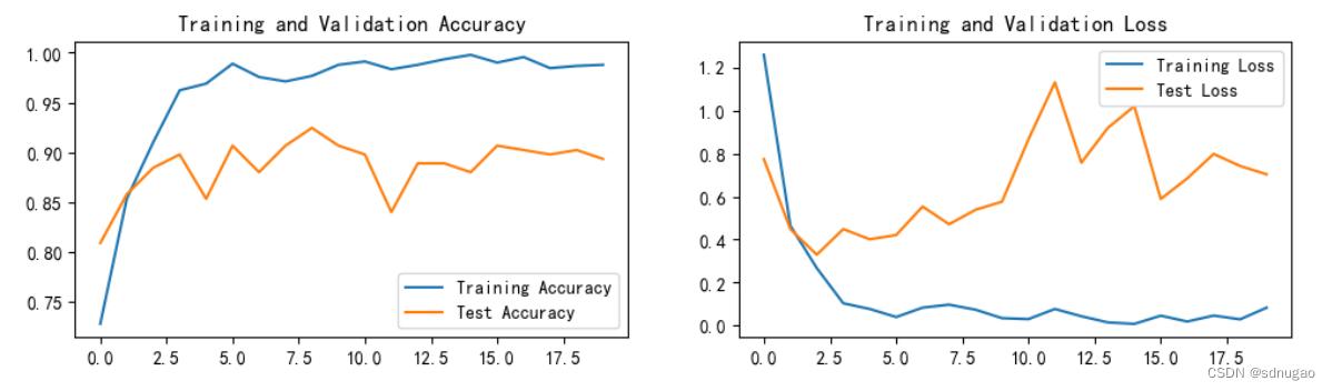
四、 结果可视化

1. Loss与Accuracy图

import matplotlib.pyplot as plt
#隐藏警告
import warnings
warnings.filterwarnings("ignore")               #忽略警告信息
plt.rcParams['font.sans-serif']    = ['SimHei'] # 用来正常显示中文标签
plt.rcParams['axes.unicode_minus'] = False      # 用来正常显示负号
plt.rcParams['figure.dpi']         = 100        #分辨率epochs_range = range(epochs)plt.figure(figsize=(12, 3))
plt.subplot(1, 2, 1)plt.plot(epochs_range, train_acc, label='Training Accuracy')
plt.plot(epochs_range, test_acc, label='Test Accuracy')
plt.legend(loc='lower right')
plt.title('Training and Validation Accuracy')plt.subplot(1, 2, 2)
plt.plot(epochs_range, train_loss, label='Training Loss')
plt.plot(epochs_range, test_loss, label='Test Loss')
plt.legend(loc='upper right')
plt.title('Training and Validation Loss')
plt.show()

2. 模型评估

best_model.eval()
epoch_test_acc, epoch_test_loss = test(test_dl, best_model, loss_fn)

epoch_test_acc, epoch_test_loss

(0.9244444444444444, 0.5387924292492579)

# 查看是否与我们记录的最高准确率一致
epoch_test_acc

0.9244444444444444