本文主要是介绍深度学习框架输出可视化中间层特征与类激活热力图,希望对大家解决编程问题提供一定的参考价值,需要的开发者们随着小编来一起学习吧!
有时候为了分析深度学习框架的中间层特征,我们需要输出中间层特征进行分析,这里提供一个方法。
(1)输出中间特征层名字
导入所需的库并加载模型
import matplotlib.pyplot as plt
import torch
import torch.nn as nn
from torch.nn import functional as F
from torchvision import transforms
import numpy as np
from PIL import Image
from collections import OrderedDict
import cv2
from models.xxx import Model  # 加载自己的模型, 这里xxx是自己模型名字
import os
device = torch.device('cuda:0')
model = Model().to(device)
print(model)
输出如下,这里我只截取了部分模型中间层输出
Model((res): ResNet50((conv1): Conv2d(3, 64, kernel_size=(7, 7), stride=(2, 2), padding=(3, 3))(maxpool): MaxPool2d(kernel_size=3, stride=2, padding=1, dilation=1, ceil_mode=False)(layer1): Sequential((0): ResNet50DownBlock((conv1): Conv2d(64, 64, kernel_size=(1, 1), stride=(1, 1))(bn1): BatchNorm2d(64, eps=1e-05, momentum=0.1, affine=True, track_running_stats=True)(conv2): Conv2d(64, 64, kernel_size=(3, 3), stride=(1, 1), padding=(1, 1))(bn2): BatchNorm2d(64, eps=1e-05, momentum=0.1, affine=True, track_running_stats=True)(conv3): Conv2d(64, 256, kernel_size=(1, 1), stride=(1, 1))(bn3): BatchNorm2d(256, eps=1e-05, momentum=0.1, affine=True, track_running_stats=True)(extra): Sequential((0): Conv2d(64, 256, kernel_size=(1, 1), stride=(1, 1))(1): BatchNorm2d(256, eps=1e-05, momentum=0.1, affine=True, track_running_stats=True)))(1): ResNet50BasicBlock((conv1): Conv2d(256, 64, kernel_size=(1, 1), stride=(1, 1))(bn1): BatchNorm2d(64, eps=1e-05, momentum=0.1, affine=True, track_running_stats=True)(conv2): Conv2d(64, 64, kernel_size=(3, 3), stride=(1, 1), padding=(1, 1))(bn2): BatchNorm2d(64, eps=1e-05, momentum=0.1, affine=True, track_running_stats=True)(conv3): Conv2d(64, 256, kernel_size=(1, 1), stride=(1, 1))(bn3): BatchNorm2d(256, eps=1e-05, momentum=0.1, affine=True, track_running_stats=True))(2): ResNet50BasicBlock((conv1): Conv2d(256, 64, kernel_size=(1, 1), stride=(1, 1))(bn1): BatchNorm2d(64, eps=1e-05, momentum=0.1, affine=True, track_running_stats=True)(conv2): Conv2d(64, 64, kernel_size=(3, 3), stride=(1, 1), padding=(1, 1))(bn2): BatchNorm2d(64, eps=1e-05, momentum=0.1, affine=True, track_running_stats=True)(conv3): Conv2d(64, 256, kernel_size=(1, 1), stride=(1, 1))(bn3): BatchNorm2d(256, eps=1e-05, momentum=0.1, affine=True, track_running_stats=True)))(layer2): Sequential((0): ResNet50DownBlock((conv1): Conv2d(256, 128, kernel_size=(1, 1), stride=(1, 1))(bn1): BatchNorm2d(128, eps=1e-05, momentum=0.1, affine=True, track_running_stats=True)(conv2): Conv2d(128, 128, kernel_size=(3, 3), stride=(2, 2), padding=(1, 1))(bn2): BatchNorm2d(128, eps=1e-05, momentum=0.1, affine=True, track_running_stats=True)(conv3): Conv2d(128, 512, kernel_size=(1, 1), stride=(1, 1))(bn3): BatchNorm2d(512, eps=1e-05, momentum=0.1, affine=True, track_running_stats=True)(extra): Sequential((0): Conv2d(256, 512, kernel_size=(1, 1), stride=(2, 2))(1): BatchNorm2d(512, eps=1e-05, momentum=0.1, affine=True, track_running_stats=True)))(1): ResNet50BasicBlock((conv1): Conv2d(512, 128, kernel_size=(1, 1), stride=(1, 1))(bn1): BatchNorm2d(128, eps=1e-05, momentum=0.1, affine=True, track_running_stats=True)(conv2): Conv2d(128, 128, kernel_size=(3, 3), stride=(1, 1), padding=(1, 1))(bn2): BatchNorm2d(128, eps=1e-05, momentum=0.1, affine=True, track_running_stats=True)(conv3): Conv2d(128, 512, kernel_size=(1, 1), stride=(1, 1))(bn3): BatchNorm2d(512, eps=1e-05, momentum=0.1, affine=True, track_running_stats=True))(2): ResNet50BasicBlock((conv1): Conv2d(512, 128, kernel_size=(1, 1), stride=(1, 1))(bn1): BatchNorm2d(128, eps=1e-05, momentum=0.1, affine=True, track_running_stats=True)(conv2): Conv2d(128, 128, kernel_size=(3, 3), stride=(1, 1), padding=(1, 1))(bn2): BatchNorm2d(128, eps=1e-05, momentum=0.1, affine=True, track_running_stats=True)(conv3): Conv2d(128, 512, kernel_size=(1, 1), stride=(1, 1))(bn3): BatchNorm2d(512, eps=1e-05, momentum=0.1, affine=True, track_running_stats=True))(3): ResNet50DownBlock((conv1): Conv2d(512, 128, kernel_size=(1, 1), stride=(1, 1))(bn1): BatchNorm2d(128, eps=1e-05, momentum=0.1, affine=True, track_running_stats=True)(conv2): Conv2d(128, 128, kernel_size=(3, 3), stride=(1, 1), padding=(1, 1))(bn2): BatchNorm2d(128, eps=1e-05, momentum=0.1, affine=True, track_running_stats=True)(conv3): Conv2d(128, 512, kernel_size=(1, 1), stride=(1, 1))(bn3): BatchNorm2d(512, eps=1e-05, momentum=0.1, affine=True, track_running_stats=True)(extra): Sequential((0): Conv2d(512, 512, kernel_size=(1, 1), stride=(1, 1))(1): BatchNorm2d(512, eps=1e-05, momentum=0.1, affine=True, track_running_stats=True))))(layer3): Sequential((0): ResNet50DownBlock((conv1): Conv2d(512, 256, kernel_size=(1, 1), stride=(1, 1))(bn1): BatchNorm2d(256, eps=1e-05, momentum=0.1, affine=True, track_running_stats=True)(conv2): Conv2d(256, 256, kernel_size=(3, 3), stride=(2, 2), padding=(1, 1))(bn2): BatchNorm2d(256, eps=1e-05, momentum=0.1, affine=True, track_running_stats=True)(conv3): Conv2d(256, 1024, kernel_size=(1, 1), stride=(1, 1))(bn3): BatchNorm2d(1024, eps=1e-05, momentum=0.1, affine=True, track_running_stats=True)(extra): Sequential((0): Conv2d(512, 1024, kernel_size=(1, 1), stride=(2, 2))(1): BatchNorm2d(1024, eps=1e-05, momentum=0.1, affine=True, track_running_stats=True)))(1): ResNet50BasicBlock((conv1): Conv2d(1024, 256, kernel_size=(1, 1), stride=(1, 1))(bn1): BatchNorm2d(256, eps=1e-05, momentum=0.1, affine=True, track_running_stats=True)(conv2): Conv2d(256, 256, kernel_size=(3, 3), stride=(1, 1), padding=(1, 1))(bn2): BatchNorm2d(256, eps=1e-05, momentum=0.1, affine=True, track_running_stats=True)(conv3): Conv2d(256, 1024, kernel_size=(1, 1), stride=(1, 1))(bn3): BatchNorm2d(1024, eps=1e-05, momentum=0.1, affine=True, track_running_stats=True))(2): ResNet50BasicBlock((conv1): Conv2d(1024, 256, kernel_size=(1, 1), stride=(1, 1))(bn1): BatchNorm2d(256, eps=1e-05, momentum=0.1, affine=True, track_running_stats=True)(conv2): Conv2d(256, 256, kernel_size=(3, 3), stride=(1, 1), padding=(1, 1))(bn2): BatchNorm2d(256, eps=1e-05, momentum=0.1, affine=True, track_running_stats=True)(conv3): Conv2d(256, 1024, kernel_size=(1, 1), stride=(1, 1))(bn3): BatchNorm2d(1024, eps=1e-05, momentum=0.1, affine=True, track_running_stats=True))(3): ResNet50DownBlock((conv1): Conv2d(1024, 256, kernel_size=(1, 1), stride=(1, 1))(bn1): BatchNorm2d(256, eps=1e-05, momentum=0.1, affine=True, track_running_stats=True)(conv2): Conv2d(256, 256, kernel_size=(3, 3), stride=(1, 1), padding=(1, 1))(bn2): BatchNorm2d(256, eps=1e-05, momentum=0.1, affine=True, track_running_stats=True)(conv3): Conv2d(256, 1024, kernel_size=(1, 1), stride=(1, 1))(bn3): BatchNorm2d(1024, eps=1e-05, momentum=0.1, affine=True, track_running_stats=True)(extra): Sequential((0): Conv2d(1024, 1024, kernel_size=(1, 1), stride=(1, 1))(1): BatchNorm2d(1024, eps=1e-05, momentum=0.1, affine=True, track_running_stats=True)))(4): ResNet50DownBlock((conv1): Conv2d(1024, 256, kernel_size=(1, 1), stride=(1, 1))(bn1): BatchNorm2d(256, eps=1e-05, momentum=0.1, affine=True, track_running_stats=True)(conv2): Conv2d(256, 256, kernel_size=(3, 3), stride=(1, 1), padding=(1, 1))(bn2): BatchNorm2d(256, eps=1e-05, momentum=0.1, affine=True, track_running_stats=True)(conv3): Conv2d(256, 1024, kernel_size=(1, 1), stride=(1, 1))(bn3): BatchNorm2d(1024, eps=1e-05, momentum=0.1, affine=True, track_running_stats=True)(extra): Sequential((0): Conv2d(1024, 1024, kernel_size=(1, 1), stride=(1, 1))(1): BatchNorm2d(1024, eps=1e-05, momentum=0.1, affine=True, track_running_stats=True)))(5): ResNet50DownBlock((conv1): Conv2d(1024, 256, kernel_size=(1, 1), stride=(1, 1))(bn1): BatchNorm2d(256, eps=1e-05, momentum=0.1, affine=True, track_running_stats=True)(conv2): Conv2d(256, 256, kernel_size=(3, 3), stride=(1, 1), padding=(1, 1))(bn2): BatchNorm2d(256, eps=1e-05, momentum=0.1, affine=True, track_running_stats=True)(conv3): Conv2d(256, 1024, kernel_size=(1, 1), stride=(1, 1))(bn3): BatchNorm2d(1024, eps=1e-05, momentum=0.1, affine=True, track_running_stats=True)(extra): Sequential((0): Conv2d(1024, 1024, kernel_size=(1, 1), stride=(1, 1))(1): BatchNorm2d(1024, eps=1e-05, momentum=0.1, affine=True, track_running_stats=True))))(2)加载并处理图像
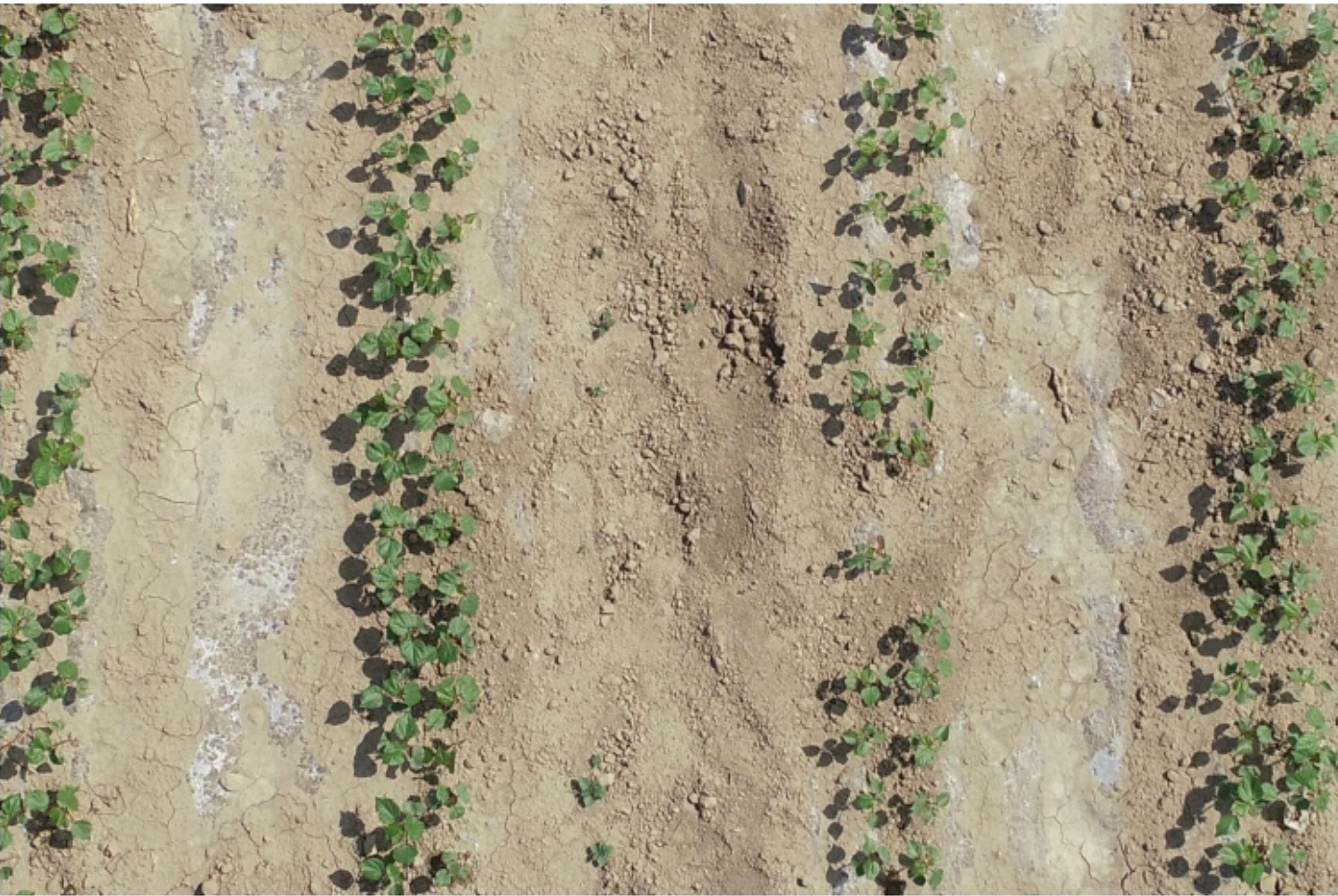
img_path = './dataset//val_data/images/100_0019_0165-11.jpg'
img = Image.open(img_path)
imgarray = np.array(img)/255.0
# plt.figure(figsize=(8, 8))
# plt.imshow(imgarray)
# plt.axis('off')
# plt.show()
加载后如下
将图片处理成模型可以预测的形式
# 处理图像
transform = transforms.Compose([transforms.Resize([512, 512]),transforms.ToTensor(),transforms.Normalize([0.485, 0.456, 0.406], [0.229, 0.224, 0.225])
])
input_img = transform(img).unsqueeze(0)  # unsqueeze(0)用于升维
# print(input_img.shape)   # torch.Size([1, 3, 512, 512])
(3)可视化中间层
1.定义钩子函数
# 定义钩子函数
activation = {}  # 保存获取的输出
def get_activation(name):def hook(model, input, output):activation[name] = output.detach()return hook
2.可视化中间层特征,这里选择了一个层,其他的自己可以类推
# 可视化中间层特征
checkpoint = torch.load('./checkpoint_best.pth') # 加载一下权重
model.load_state_dict(checkpoint['model'])
model.eval()
model.res.layer1[2].register_forward_hook(get_activation('bn3')) #resnet50 layer1中第三个模块的bn3注册钩子
input_img = input_img.to(device) # cpu数据转一下gpu,这个看你会不会报错,我的不转会报错
_ = model(input_img)
bn3 = activation['bn3'] # 结果将保存在activation字典中 bn3输出<class 'torch.Tensor'>, tensor是无法用plt正常显示的
# print(bn3.shape) # 调试到这里基本成功了
bn3 = bn3.cpu().numpy() # 转一下numpy, shape:(1,256, 128, 128)
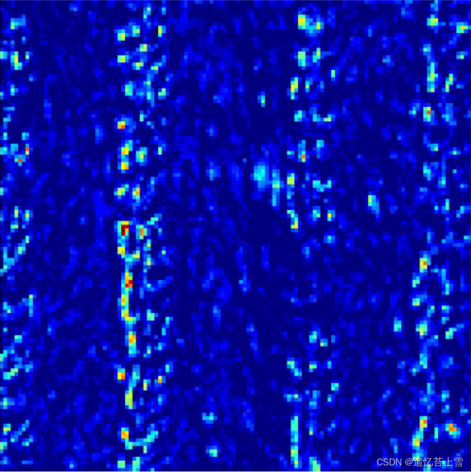
plt.figure(figsize=(8,8))
plt.imshow(bn3[0][0], cmap='gray') # bn3[0][0] shape:(128, 128)
plt.axis('off')
# # shape:(128, 128)
plt.show()可视化结果
(4)利用循环输出多张图像可视化中间层
整合上面的代码,利用循环输出验证集中的多张图像中的可视化中间层
# 加载依赖包
import matplotlib.pyplot as plt
import torch
import torch.nn as nn
from torch.nn import functional as F
from torchvision import transforms
import numpy as np
from PIL import Image
from collections import OrderedDict
import cv2
from models.M_SFANet import Model
import os
import glob# 定义钩子函数
activation = {}  # 保存获取的输出
def get_activation(name):def hook(model, input, output):activation[name] = output.detach()return hook# 加载模型
device = torch.device('cuda:0')
model = Model().to(device)checkpoint = torch.load('./checkpoint_best.pth')  # 加载一下权重
model.load_state_dict(checkpoint['model'])
model.eval()
model.res.layer1[2].register_forward_hook(get_activation('bn3'))  #resnet50 layer1中第三个模块的bn3注册钩子,如果需要其他层数就用其他的# 利用循环输出多个可视化中间层#读取需要输出特征的图像
DATA_PATH = f"./val_data/"
img_list = glob.glob(os.path.join(DATA_PATH, "images", "*.jpg"))    # image 路径
img_list.sort()
for idx in range(0, len(img_list)):img_name = img_list[idx].split('/')[-1].split('.')[0]  # 获取文件名img = Image.open(img_list[idx])  # 可以读到图片imgarray = np.array(img)/255.0# 处理图像transform = transforms.Compose([transforms.Resize([512, 512]),transforms.ToTensor(),transforms.Normalize([0.485, 0.456, 0.406], [0.229, 0.224, 0.225])])input_img = transform(img).unsqueeze(0)  # unsqueeze(0)用于升维input_img = input_img.to(device)  # cpu数据转一下gpu,这个看你会不会报错,我的会报错_ = model(input_img)bn3 = activation['bn3']   # 结果将保存在activation字典中  bn3输出<class 'torch.Tensor'>, tensor是无法用plt正常显示的bn3 = bn3.cpu().numpy() plt.figure(figsize=(8,8))plt.imshow(bn3[0][0], cmap='jet')  # bn3[0][0]  shape:(128, 128)plt.axis('off')# # shape:(128, 128)plt.savefig('./feature_out/res50/layer1/{}_res50_layer1'.format(img_name), bbox_inches='tight', pad_inches=0.05, dpi=300)
保存至文件夹中如下
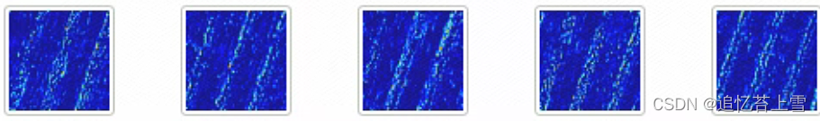
---------------------------------------------------更新于2023.1121.28 -----------------------------------------
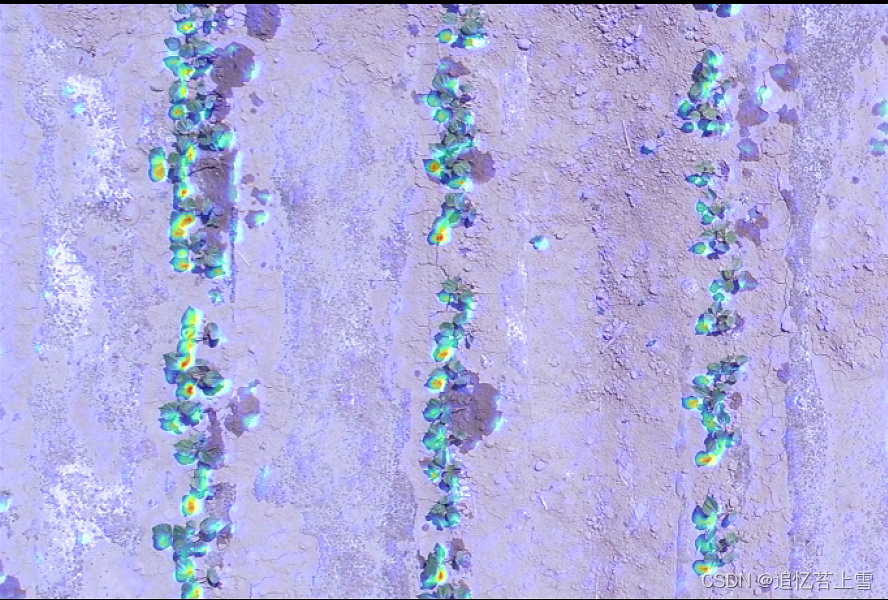
(5)利用循环输出多张图像类激活热力图
使用类激活热力图,能观察模型对图像识别的关键位置。
这里接着上面的获得的特征图进一步得到类激活热力图
接着上面获取到bn3,代码如下
bn3 = activation['bn3'] # 结果将保存在activation字典中 bn3输出<class 'torch.Tensor'>, tensor是无法用plt正常显示的'''以下代码用于输出特征图bn3 = bn3.cpu().numpy() plt.figure(figsize=(8,8))plt.imshow(bn3[0][0], cmap='jet') # bn3[0][0] shape:(128, 128)plt.axis('off')# # shape:(128, 128)plt.savefig('./feature_out/res50/layer4/{}_res50_layer4'.format(img_name), bbox_inches='tight', pad_inches=0.05, dpi=300)'''# 将特征图用类热力图形式叠加到原图中bn3 = bn3[0][0].cpu().numpy()bn3 = np.maximum(bn3, 0)bn3 /= np.max(bn3)# plt.matshow(bn3)# plt.show()# img1 = cv2.imread('./dataset/ShanghaiTech/part_A_final/val_data/images/100_0019_0165-11.jpg')img1 = cv2.cvtColor(np.asarray(img), cv2.COLOR_RGB2BGR) # PIL Image转一下cv2bn3 = cv2.resize(bn3, (img1.shape[1], img1.shape[0]))bn3 = np.uint8(255 * bn3)bn3 = cv2.applyColorMap(bn3, cv2.COLORMAP_JET)heat_img = cv2.addWeighted(img1, 1, bn3, 0.5, 0)cv2.imwrite('./heatmap_out/res50/layer1/{}_res50_layer1.jpg'.format(str(img_name)), heat_img)输出如下
这篇关于深度学习框架输出可视化中间层特征与类激活热力图的文章就介绍到这儿,希望我们推荐的文章对编程师们有所帮助!


