nvidia-rapids︱cuML机器学习加速库

本文主要是介绍nvidia-rapids︱cuML机器学习加速库，希望对大家解决编程问题提供一定的参考价值，需要的开发者们随着小编来一起学习吧！

cuML是一套用于实现与其他RAPIDS项目共享兼容API的机器学习算法和数学原语函数。

cuML使数据科学家、研究人员和软件工程师能够在GPU上运行传统的表格ML任务，而无需深入了解CUDA编程的细节。 在大多数情况下，cuML的Python API与来自scikit-learn的API相匹配。

对于大型数据集，这些基于GPU的实现可以比其CPU等效完成10-50倍。 有关性能的详细信息，请参阅cuML基准测试笔记本。

官方文档：
rapidsai/cuml
cuML API Reference

官方案例还是蛮多的：

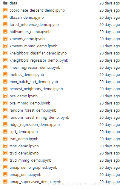
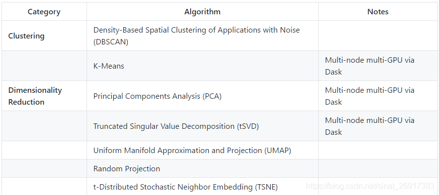
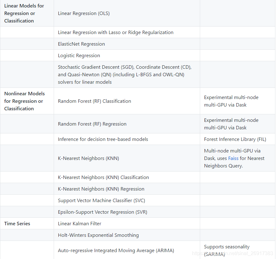
来看看有啥模型：

关联文章：

nvidia-rapids︱cuDF与pandas一样的DataFrame库
NVIDIA的python-GPU算法生态 ︱ RAPIDS 0.10
nvidia-rapids︱cuML机器学习加速库
nvidia-rapids︱cuGraph(NetworkX-like)关系图模型

---

---

1 安装与背景

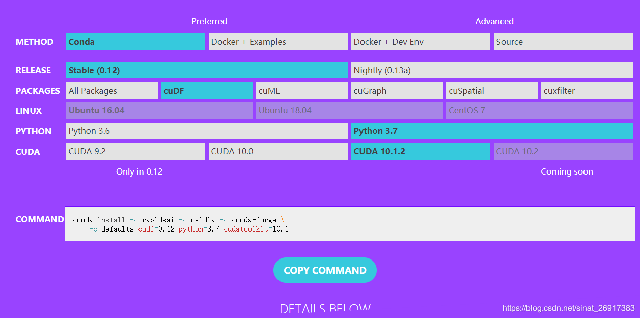
1.1 安装

参考：https://github.com/rapidsai/cuml/blob/branch-0.13/BUILD.md

conda env create -n cuml_dev python=3.7 --file=conda/environments/cuml_dev_cuda10.0.yml

docker版本，可参考：https://rapids.ai/start.html#prerequisites

docker pull rapidsai/rapidsai:cuda10.1-runtime-ubuntu16.04-py3.7
docker run --gpus all --rm -it -p 8888:8888 -p 8787:8787 -p 8786:8786 \rapidsai/rapidsai:cuda10.1-runtime-ubuntu16.04-py3.7

1.2 背景

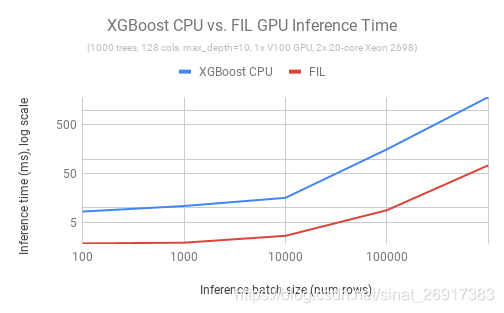
不仅是训练，要想真正在GPU上扩展数据科学，也需要加速端到端的应用程序。cuML 0.9 为我们带来了基于GPU的树模型支持的下一个发展，包括新的森林推理库（FIL）。FIL是一个轻量级的GPU加速引擎，它对基于树形模型进行推理，包括梯度增强决策树和随机森林。使用单个V100 GPU和两行Python代码，用户就可以加载一个已保存的XGBoost或LightGBM模型，并对新数据执行推理，速度比双20核CPU节点快36倍。在开源Treelite软件包的基础上，下一个版本的FIL还将添加对scikit-learn和cuML随机森林模型的支持。

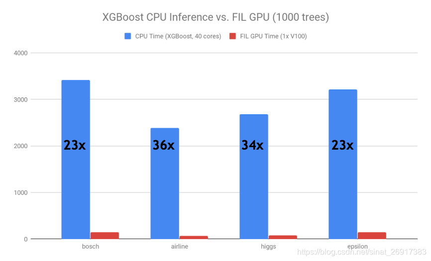
图3：推理速度对比，XGBoost CPU vs 森林推理库 (FIL) GPU

---

2 DBSCAN

The DBSCAN algorithm is a clustering algorithm that works really well for datasets that have regions of high density.

The model can take array-like objects, either in host as NumPy arrays or in device (as Numba or cuda_array_interface-compliant), as well as cuDF DataFrames.

import cudf
import matplotlib.pyplot as plt
import numpy as np
from cuml.datasets import make_blobs
from cuml.cluster import DBSCAN as cuDBSCAN
from sklearn.cluster import DBSCAN as skDBSCAN
from sklearn.metrics import adjusted_rand_score%matplotlib inline# 定义参数
n_samples = 10**4
n_features = 2eps = 0.15
min_samples = 3
random_state = 23#Generate Data
%%time
device_data, device_labels = make_blobs(n_samples=n_samples, n_features=n_features,centers=5,cluster_std=0.1,random_state=random_state)device_data = cudf.DataFrame.from_gpu_matrix(device_data)
device_labels = cudf.Series(device_labels)
# Copy dataset from GPU memory to host memory.
# This is done to later compare CPU and GPU results.
host_data = device_data.to_pandas()
host_labels = device_labels.to_pandas()# sklearn 模型拟合
%%time
clustering_sk = skDBSCAN(eps=eps,min_samples=min_samples,algorithm="brute",n_jobs=-1)clustering_sk.fit(host_data)# cuML 模型拟合
%%time
clustering_cuml = cuDBSCAN(eps=eps,min_samples=min_samples,verbose=True,max_mbytes_per_batch=13e3)clustering_cuml.fit(device_data, out_dtype="int32")# 可视化
fig = plt.figure(figsize=(16, 10))X = np.array(host_data)
labels = clustering_cuml.labels_n_clusters_ = len(labels)# Black removed and is used for noise instead.
unique_labels = labels.unique()
colors = [plt.cm.Spectral(each)for each in np.linspace(0, 1, len(unique_labels))]
for k, col in zip(unique_labels, colors):if k == -1:# Black used for noise.col = [0, 0, 0, 1]class_member_mask = (labels == k)xy = X[class_member_mask]plt.plot(xy[:, 0], xy[:, 1], 'o', markerfacecolor=tuple(col),markersize=5, markeredgecolor=tuple(col))plt.title('Estimated number of clusters: %d' % n_clusters_)
plt.show()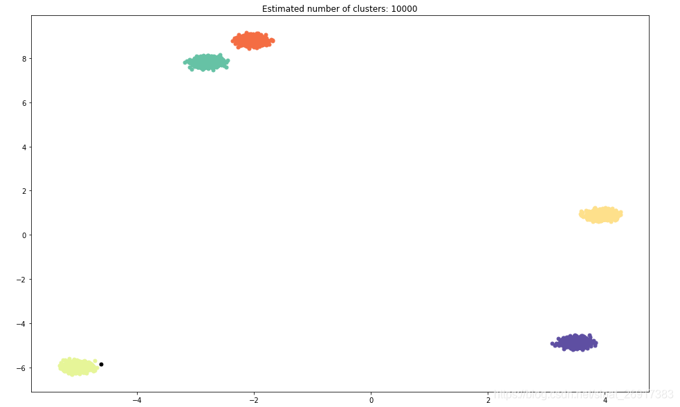

结果评估：

%%time
sk_score = adjusted_rand_score(host_labels, clustering_sk.labels_)
cuml_score = adjusted_rand_score(host_labels, clustering_cuml.labels_)>>> (0.9998750031236718, 0.9998750031236718)

两个结果是一模一样的，也就是skearn和cuML的结果一致。

---

3 TSNE算法在Fashion MNIST的使用

TSNE (T-Distributed Stochastic Neighborhood Embedding) is a fantastic dimensionality reduction algorithm used to visualize large complex datasets including medical scans, neural network weights, gene expressions and much more.

cuML’s TSNE algorithm supports both the faster Barnes Hut $ n logn $ algorithm and also the slower Exact $ n^2 $ .

The model can take array-like objects, either in host as NumPy arrays as well as cuDF DataFrames as the input.

import gzip
import matplotlib.pyplot as plt
import numpy as np
import os
from cuml.manifold import TSNE%matplotlib inline# https://github.com/zalandoresearch/fashion-mnist/blob/master/utils/mnist_reader.py
def load_mnist_train(path):"""Load MNIST data from path"""labels_path = os.path.join(path, 'train-labels-idx1-ubyte.gz')images_path = os.path.join(path, 'train-images-idx3-ubyte.gz')with gzip.open(labels_path, 'rb') as lbpath:labels = np.frombuffer(lbpath.read(), dtype=np.uint8,offset=8)with gzip.open(images_path, 'rb') as imgpath:images = np.frombuffer(imgpath.read(), dtype=np.uint8,offset=16).reshape(len(labels), 784)return images, labels# 加载数据
images, labels = load_mnist_train("data/fashion")plt.figure(figsize=(5,5))
plt.imshow(images[100].reshape((28, 28)), cmap = 'gray')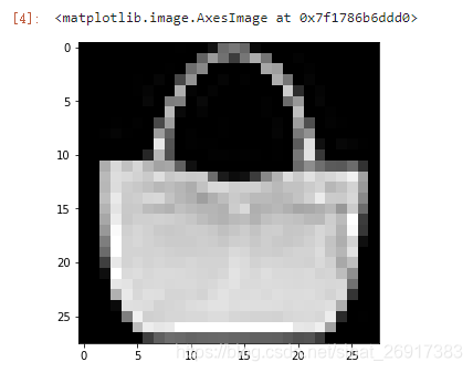

# 建模
tsne = TSNE(n_components = 2, method = 'barnes_hut', random_state=23)
%time embedding = tsne.fit_transform(images)print(embedding[:10], embedding.shape)CPU times: user 2.41 s, sys: 2.57 s, total: 4.98 s
Wall time: 4.98 s
[[-13.577632    39.87483   ][ 26.136728   -17.68164   ][ 23.164072    22.151243  ][ 28.361032    11.134571  ][ 35.419216     5.6633983 ][ -0.15575314 -11.143476  ][-24.30308     -1.584903  ][ -5.9438944  -27.522072  ][  2.0439444   29.574451  ][ -3.0801039   27.079374  ]] (60000, 2)

可视化Visualize Embedding：

# Visualize Embeddingclasses = ['T-shirt/top','Trouser','Pullover','Dress','Coat','Sandal','Shirt','Sneaker','Bag','Ankle boot'
]fig, ax = plt.subplots(1, figsize = (14, 10))
plt.scatter(embedding[:,1], embedding[:,0], s = 0.3, c = labels, cmap = 'Spectral')
plt.setp(ax, xticks = [], yticks = [])
cbar = plt.colorbar(boundaries = np.arange(11)-0.5)
cbar.set_ticks(np.arange(10))
cbar.set_ticklabels(classes)
plt.title('Fashion MNIST Embedded via TSNE');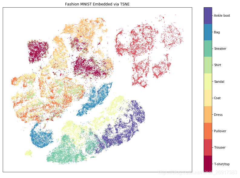

---

4 XGBoosting

import numpy as np; print('numpy Version:', np.__version__)
import pandas as pd; print('pandas Version:', pd.__version__)
import xgboost as xgb; print('XGBoost Version:', xgb.__version__)# helper function for simulating data
def simulate_data(m, n, k=2, numerical=False):if numerical:features = np.random.rand(m, n)else:features = np.random.randint(2, size=(m, n))labels = np.random.randint(k, size=m)return np.c_[labels, features].astype(np.float32)# helper function for loading data
def load_data(filename, n_rows):if n_rows >= 1e9:df = pd.read_csv(filename)else:df = pd.read_csv(filename, nrows=n_rows)return df.values.astype(np.float32)# settings
LOAD = False
n_rows = int(1e5)
n_columns = int(100)
n_categories = 2# 加载数据
%%timeif LOAD:dataset = load_data('/tmp', n_rows)
else:dataset = simulate_data(n_rows, n_columns, n_categories)
print(dataset.shape)# 训练集切分
# identify shape and indices
n_rows, n_columns = dataset.shape
train_size = 0.80
train_index = int(n_rows * train_size)# split X, y
X, y = dataset[:, 1:], dataset[:, 0]
del dataset# split train data
X_train, y_train = X[:train_index, :], y[:train_index]# split validation data
X_validation, y_validation = X[train_index:, :], y[train_index:]# 检验
# check dimensions
print('X_train: ', X_train.shape, X_train.dtype, 'y_train: ', y_train.shape, y_train.dtype)
print('X_validation', X_validation.shape, X_validation.dtype, 'y_validation: ', y_validation.shape, y_validation.dtype)# check the proportions
total = X_train.shape[0] + X_validation.shape[0]
print('X_train proportion:', X_train.shape[0] / total)
print('X_validation proportion:', X_validation.shape[0] / total)# Convert NumPy data to DMatrix format
%%timedtrain = xgb.DMatrix(X_train, label=y_train)
dvalidation = xgb.DMatrix(X_validation, label=y_validation)# 设置参数
# instantiate params
params = {}# general params
general_params = {'silent': 1}
params.update(general_params)# booster params
n_gpus = 1
booster_params = {}if n_gpus != 0:booster_params['tree_method'] = 'gpu_hist'booster_params['n_gpus'] = n_gpus
params.update(booster_params)# learning task params
learning_task_params = {'eval_metric': 'auc', 'objective': 'binary:logistic'}
params.update(learning_task_params)
print(params)# 模型训练
# model training settings
evallist = [(dvalidation, 'validation'), (dtrain, 'train')]
num_round = 10%%timebst = xgb.train(params, dtrain, num_round, evallist)

输出：

[0]	validation-auc:0.504014	train-auc:0.542211
[1]	validation-auc:0.506166	train-auc:0.559262
[2]	validation-auc:0.501638	train-auc:0.570375
[3]	validation-auc:0.50275	train-auc:0.580726
[4]	validation-auc:0.503445	train-auc:0.589701
[5]	validation-auc:0.503413	train-auc:0.598342
[6]	validation-auc:0.504258	train-auc:0.605253
[7]	validation-auc:0.503157	train-auc:0.611937
[8]	validation-auc:0.502372	train-auc:0.617561
[9]	validation-auc:0.501949	train-auc:0.62333
CPU times: user 1.12 s, sys: 195 ms, total: 1.31 s
Wall time: 360 ms

相关参考：

• Open Source Website
• GitHub
• Press Release
• NVIDIA Blog
• Developer Blog
• NVIDIA Data Science Webpage

---

5 利用KNN进行图像检索

参考：在GPU实例上使用RAPIDS加速图像搜索任务

阿里云文档中有专门的介绍，所以不做太多赘述。
使用开源框架Tensorflow和Keras提取图片特征，其中模型为基于ImageNet数据集的ResNet50（notop）预训练模型。
连接公网下载模型（大小约91M），下载完成后默认保存到/root/.keras/models/目录

数据下载：

import os
import tarfile
import numpy as np
from urllib.request import urlretrievedef download_and_extract(data_dir):"""doc"""def _progress(count, block_size, total_size):print('\r>>> Downloading %s  (total:%.0fM) %.1f%%' % (filename, total_size / 1024 / 1024, 100.0 * count * block_size / total_size), end='')url = 'http://ai.stanford.edu/~acoates/stl10/stl10_binary.tar.gz'filename = url.split('/')[-1]filepath = os.path.join(data_dir, filename)decom_dir = os.path.join(data_dir, filename.split('.')[0])if not os.path.exists(data_dir):os.makedirs(data_dir)if os.path.exists(filepath):print('>>> {} has exist in current directory.'.format(filename))else:urlretrieve(url, filepath, _progress)print("\nSuccessfully downloaded.")if not os.path.exists(decom_dir):# Decompressprint(">>> Decompressing from {}....".format(filepath))tar = tarfile.open(filepath, 'r')tar.extractall(data_dir)print("Successfully decompressed")tar.close()else:print('>>> Directory "{}" has exist. '.format(decom_dir))def read_all_images(path_to_data):"""get all images from binary path"""with open(path_to_data, 'rb') as f:everything = np.fromfile(f, dtype=np.uint8)images = np.reshape(everything, (-1, 3, 96, 96))images = np.transpose(images, (0, 3, 2, 1))return images# the directory to save data
data_dir = './data'
# download and decompression
download_and_extract(data_dir)# 读入数据
# the path of unlabeled data
path_unlabeled = os.path.join(data_dir, 'stl10_binary/unlabeled_X.bin')
# get images from binary
images = read_all_images(path_unlabeled)
print('>>> images shape: ', images.shape)# 看图
import random
import matplotlib.pyplot as plt
%matplotlib inlinedef show_image(image):"""show image"""fig = plt.figure(figsize=(3, 3))plt.imshow(image)plt.show()fig.clear()# random show a image
rand_image_index = random.randint(0, images.shape[0])
show_image(images[rand_image_index])

# 分割数据
from sklearn.model_selection import train_test_splittrain_images, query_images = train_test_split(images, test_size=0.1, random_state=123)
print('train_images shape: ', train_images.shape)
print('query_images shape: ', query_images.shape)# 图片特征
# set tensorflow params to adjust GPU memory usage, if use default params, tensorflow would use
# nearly all of the gpu memory, we need reserve some gpu memory for cuml.
import os
# only use device 0
os.environ["CUDA_VISIBLE_DEVICES"] = "0"import tensorflow as tf
from keras.backend.tensorflow_backend import set_session
config = tf.ConfigProto()
# method 1: allocate gpu memory base on runtime allocations
# config.gpu_options.allow_growth = True
# method 2: determines the fraction of the onerall amount of memory 
# that each visibel GPU should be allocated.
config.gpu_options.per_process_gpu_memory_fraction = 0.3
set_session(tf.Session(config=config))# 特征抽取
from keras.applications.resnet50 import ResNet50
from keras.preprocessing import image
from keras.applications.resnet50 import preprocess_input# download resnet50(notop) model(first running) and load model
model = ResNet50(weights='imagenet', include_top=False, input_shape=(96, 96, 3), pooling='max')
# network summary
model.summary()%%time
train_features = model.predict(train_images)
print('train features shape: ', train_features.shape)%%time
query_features = model.predict(query_images)
print('query features shape: ', query_features.shape)

然后是KNN阶段,包括了sklear-KNN，和CUML-KNN：

from cuml.neighbors import NearestNeighbors%%time
knn_cuml = NearestNeighbors()
knn_cuml.fit(train_features)%%time
distances_cuml, indices_cuml = knn_cuml.kneighbors(query_features, k=3)from sklearn.neighbors import NearestNeighbors
%%time
knn_sk = NearestNeighbors(n_neighbors=3, metric='sqeuclidean', n_jobs=-1)
knn_sk.fit(train_features)%%time
distances_sk, indices_sk = knn_sk.kneighbors(query_features, 3)
# compare the distance obtained while using sklearn and cuml models
(np.abs(distances_cuml - distances_sk) < 1).all()# 展示结果
def show_images(query, sim_images, sim_dists):"""doc"""simi_num = len(sim_images)fig = plt.figure(figsize=(3 * (simi_num + 1), 3))axes = fig.subplots(1, simi_num + 1)for index, ax in enumerate(axes):if index == 0:ax.imshow(query)ax.set_title('query')else:ax.imshow(sim_images[index - 1])ax.set_title('dist: %.1f' % (sim_dists[index - 1]))plt.show()fig.clear()# get random indices
random_show_index = np.random.randint(0, query_images.shape[0], size=5)
random_query = query_images[random_show_index]
random_indices = indices_cuml[random_show_index].astype(np.int)
random_distances = distances_cuml[random_show_index]# show result images
for query_image, sim_indices, sim_dists in zip(random_query, random_indices, random_distances):sim_images = train_images[sim_indices]show_images(query_image, sim_images, sim_dists)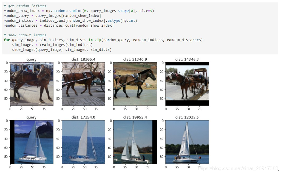

---

用到后再追加..

这篇关于nvidia-rapids︱cuML机器学习加速库的文章就介绍到这儿，希望我们推荐的文章对编程师们有所帮助！

---