本文主要是介绍深度学习TensorFlow2基础知识学习前半部分,希望对大家解决编程问题提供一定的参考价值,需要的开发者们随着小编来一起学习吧!
目录
测试TensorFlow是否支持GPU:
自动求导:
数据预处理 之 统一数组维度
定义变量和常量
训练模型的时候设备变量的设置
生成随机数据
交叉熵损失CE和均方误差函数MSE
全连接Dense层
维度变换reshape
增加或减小维度
数组合并
广播机制:
简单范数运算
矩阵转置
框架本身只是用来编写的工具,每个框架包括Pytorch,tensorflow、mxnet、paddle、mandspore等等框架编程语言上其实差别是大同小异的,不同的点是他们在编译方式、运行方式或者计算速度上,我也浅浅的学习一下这个框架以便于看github上的代码可以轻松些。
我的环境:
google colab的T4 GPU
首先是
测试TensorFlow是否支持GPU:
打开tf的config包,里面有个list_pysical_devices("GPU")
import os
import tensorflow as tfos.environ['TF_CPP_Min_LOG_LEVEL']='3'
os.system("clear")
print("GPU列表:",tf.config.list_logical_devices("GPU"))
运行结果:
GPU列表: [LogicalDevice(name='/device:GPU:0', device_type='GPU')]

检测运行时间:
def run():n=1000#CPU计算矩阵with tf.device('/cpu:0'):cpu_a = tf.random.normal([n,n])cpu_b = tf.random.normal([n,n])print(cpu_a.device,cpu_b.device)#GPU计算矩阵with tf.device('/gpu:0'):gpu_a = tf.random.normal([n,n])gpu_b = tf.random.normal([n,n])print(gpu_a.device,gpu_b.device)def cpu_run():with tf.device('/cpu:0'):c = tf.matmul(cpu_a,cpu_b)return cdef gpu_run():with tf.device('/cpu:0'):c = tf.matmul(gpu_a,gpu_b)return cnumber=1000print("初次运行:")cpu_time=timeit.timeit(cpu_run,number=number)gpu_time=timeit.timeit(gpu_run,number=number)print("cpu计算时间:",cpu_time)print("Gpu计算时间:",gpu_time)print("再次运行:")cpu_time=timeit.timeit(cpu_run,number=number)gpu_time=timeit.timeit(gpu_run,number=number)print("cpu计算时间:",cpu_time)print("Gpu计算时间:",gpu_time)run()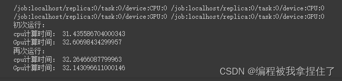
可能T4显卡不太好吧...体现不出太大的效果,也可能是GPU在公用或者还没热身。
自动求导:
公式:
f(x)=x^n微分(导数):
f'(x)=n*x^(n-1)例:
y=x^2
微分(导数):
dy/dx=2x^(2-1)=2x
x = tf.constant(10.)   # 定义常数变量值
with tf.GradientTape() as tape:   #调用tf底下的求导函数tape.watch([x])   # 使用tape.watch()去观察和跟踪watchy=x**2dy_dx = tape.gradient(y,x)
print(dy_dx)
运行结果:tf.Tensor(20.0, shape=(), dtype=float32)
数据预处理 之 统一数组维度
对拿到的脏数据进行预处理的时候需要进行统一数组维度操作,使用tensorflow.keras.preprocessing.sequence 底下的pad_sequences函数,比如下面有三个不等长的数组,我们需要对数据处理成相同的长度,可以进行左边或者补个数
import numpy as np
import pprint as pp #让打印出来的更加好看
from tensorflow.keras.preprocessing.sequence import pad_sequencescomment1 = [1,2,3,4]
comment2 = [1,2,3,4,5,6,7]
comment3 = [1,2,3,4,5,6,7,8,9,10]x_train = np.array([comment1, comment2, comment3], dtype=object)
print(), pp.pprint(x_train)# 左补0,统一数组长度
x_test = pad_sequences(x_train)
print(), pp.pprint(x_test)# 左补255,统一数组长度
x_test = pad_sequences(x_train, value=255)
print(), pp.pprint(x_test)# 右补0,统一数组长度
x_test = pad_sequences(x_train, padding="post")
print(), pp.pprint(x_test)# 切取数组长度, 只保留后3位
x_test = pad_sequences(x_train, maxlen=3)
print(), pp.pprint(x_test)# 切取数组长度, 只保留前3位
x_test = pad_sequences(x_train, maxlen=3, truncating="post")
print(), pp.pprint(x_test)
array([list([1, 2, 3, 4]), list([1, 2, 3, 4, 5, 6, 7]),list([1, 2, 3, 4, 5, 6, 7, 8, 9, 10])], dtype=object)array([[ 0, 0, 0, 0, 0, 0, 1, 2, 3, 4],[ 0, 0, 0, 1, 2, 3, 4, 5, 6, 7],[ 1, 2, 3, 4, 5, 6, 7, 8, 9, 10]], dtype=int32)array([[255, 255, 255, 255, 255, 255, 1, 2, 3, 4],[255, 255, 255, 1, 2, 3, 4, 5, 6, 7],[ 1, 2, 3, 4, 5, 6, 7, 8, 9, 10]], dtype=int32)array([[ 1, 2, 3, 4, 0, 0, 0, 0, 0, 0],[ 1, 2, 3, 4, 5, 6, 7, 0, 0, 0],[ 1, 2, 3, 4, 5, 6, 7, 8, 9, 10]], dtype=int32)array([[ 2, 3, 4],[ 5, 6, 7],[ 8, 9, 10]], dtype=int32)array([[1, 2, 3],[1, 2, 3],[1, 2, 3]], dtype=int32)(None, None)
定义变量和常量
tf中变量定义为Variable,常量Tensor(这里懂了吧,pytorch里面都是Tensor,但是tf里面的Tensor代表向量其实也是可变的),要注意的是Variable数组和变量数值之间的加减乘除可以进行广播机制的运算,而且常量和变量之间也是可以相加的。
import os
os.environ['TF_CPP_MIN_LOG_LEVEL'] = '3'
os.system("cls")import tensorflow as tf################################
# 定义变量
a = tf.Variable(1)
b = tf.Variable(1.)
c = tf.Variable([1.])
d = tf.Variable(1., dtype=tf.float32)print("-" * 40)
print(a)
print(b)
print(c)
print(d)# print(a+b)  # error:类型不匹配
print(b+c)    # 注意这里是Tensor类型
print(b+c[0]) # 注意这里是Tensor类型################################
# 定义Tensor
x1 = tf.constant(1)
x2 = tf.constant(1.)
x3 = tf.constant([1.])
x4 = tf.constant(1, dtype=tf.float32)print("-" * 40)
print(x1)
print(x2)
print(x3)
print(x4)print(x2+x3[0])
运行结果:
----------------------------------------
<tf.Variable 'Variable:0' shape=() dtype=int32, numpy=1> <tf.Variable 'Variable:0' shape=() dtype=float32, numpy=1.0> <tf.Variable 'Variable:0' shape=(1,) dtype=float32, numpy=array([1.], dtype=float32)> <tf.Variable 'Variable:0' shape=() dtype=float32, numpy=1.0> tf.Tensor([2.], shape=(1,), dtype=float32) tf.Tensor(2.0, shape=(), dtype=float32)
----------------------------------------
tf.Tensor(1, shape=(), dtype=int32) tf.Tensor(1.0, shape=(), dtype=float32) tf.Tensor([1.], shape=(1,), dtype=float32) tf.Tensor(1.0, shape=(), dtype=float32) tf.Tensor(2.0, shape=(), dtype=float32)
训练模型的时候设备变量的设置
使用Variable:
如果定义整数默认定义在CPU,定义浮点数默认在GPU上,但是咱们在tf2.0上不用去关心他的变量类型,因为2.0进行运算的变量都在GPU上进行运算(前提上本地有GPU).
使用identity指定变量所定义的设备,在2.0其实不用管了,1.0可能代码得有两个不同设备的版本,但在2.0就不需要在意这个问题了。
################################
# 定义变量后看设备
a = tf.Variable(1)
b = tf.Variable(10.)print("-" * 40)
print("a.device:", a.device, a) # CPU
print("b.device:", b.device, b) # GPU################################
# 定义Tensor后看设备
x1 = tf.constant(100)
x2 = tf.constant(1000.)print("-" * 40)
print("x1.device:", x1.device, x1) # CPU
print("x2.device:", x2.device, x2) # CPU################################
print("-" * 40)# CPU+CPU
ax1 = a + x1
print("ax1.device:", ax1.device, ax1) # GPU# CPU+GPU
bx2 = b + x2
print("bx2.device:", bx2.device, bx2) # GPU################################
# 指定GPU设备定义Tensor
gpu_a = tf.identity(a)
gpu_x1 = tf.identity(x1)print("-" * 40)
print("gpu_a.device:", gpu_a.device, gpu_a)
print("gpu_x1.device:", gpu_x1.device, gpu_x1)
生成随机数据
其实tf和numpy在创建上是大同小异的,除了变量类型不一样。
a = np.ones(12)
print(a)
a = tf.convert_to_tensor(a)#其实没必要转换,直接像下面的方法进行定义。
a = tf.zeros(12)
a = tf.zeros([4,3])
a = tf.zeros([4,6,3])
b = tf.zeros_like(a)
a = tf.ones(12)
a = tf.ones_like(b)
a = tf.fill([3,2], 10.)
a = tf.random.normal([12])
a = tf.random.normal([4,3])
a = tf.random.truncated_normal([3,2])
a = tf.random.uniform([4,3], minval=0, maxval=10)
a = tf.random.uniform([12], minval=0, maxval=10, dtype=tf.int32)
a = tf.range([12], dtype=tf.int32)
b = tf.random.shuffle(a)
print(b)
代码我就不贴了。
交叉熵损失CE和均方误差函数MSE
假设batch=1
直接看怎么用,以图像分类为例,输出是类别个数,选择最大神经原的下标,然后进行独热编码把它变成[1,0,0,0,...],然后就可以与softmax之后的输出概率值之间做交叉熵损失。
rows = 1
out = tf.nn.softmax(tf.random.uniform([rows,2]),axis=1)
print("out:", out)
print("预测值:", tf.math.argmax(out, axis=1), "\n")y = tf.range(rows)
print("y:", y, "\n")y = tf.one_hot(y, depth=10)
print("y_one_hot:", y, "\n")loss = tf.keras.losses.binary_crossentropy(y,out)
# loss = tf.keras.losses.mse(y, out)
print("row loss", loss, "\n")
假设batch=2
rows = 2
out = tf.random.uniform([rows,1])
print("预测值:", out, "\n")y = tf.constant([1])
print("y:", y, "\n")# y = tf.one_hot(y, depth=1)print("y_one_hot:", y, "\n")loss = tf.keras.losses.mse(y,out)
# loss = tf.keras.losses.mse(y, out)
print("row loss", loss, "\n")loss = tf.reduce_mean(loss)
print("总体损失:", loss, "\n")
总损失就是一个batch的损失求均值。
全连接Dense层
###################################################
# Dense: y=wx+b
rows = 1
net = tf.keras.layers.Dense(1) # 一个隐藏层,一个神经元
net.build((rows, 1)) # (编译)每个训练数据有1个特征
print("net.w:", net.kernel) # 参数个数
print("net.b:", net.bias) # 和Dense数一样
假设有一个特征输出,如果讲bulid参数改成(rows,3),那么神经元个数的w参数输出就变成了(3,1)大小的数据。
维度变换reshape
跟numpy一毛一样不用看了
# 10张彩色图片
a = tf.random.normal([10,28,28,3])
print(a)
print(a.shape) # 形状
print(a.ndim)  # 维度b = tf.reshape(a, [10, 784, 3])
print(b)
print(b.shape) # 形状
print(b.ndim)  # 维度c = tf.reshape(a, [10, -1, 3])
print(c)
print(c.shape) # 形状
print(c.ndim)  # 维度d = tf.reshape(a, [10, 784*3])
print(d)
print(d.shape) # 形状
print(d.ndim)  # 维度e = tf.reshape(a, [10, -1])
print(e)
print(e.shape) # 形状
print(e.ndim)  # 维度
增加或减小维度
a = tf.range([24])
# a = tf.reshape(a, [4,6])
print(a)
print(a.shape)
print(a.ndim)# 增加一个维度,相当于[1,2,3]->[[1,2,3]]
b = tf.expand_dims(a, axis=0)
print(b)
print(b.shape)
print(b.ndim)# 减少维度,相当于[[1,2,3]]->[1,2,3]
c = tf.squeeze(b, axis=0)
print(c)
print(c.shape)
print(c.ndim)
数组合并
真t和numpy一毛一样
####################################################
# 数组合并
# tf.concat
a = tf.zeros([2,4,3])
b = tf.ones([2,4,3])print(a)
print(b)# 0轴合并,4,4,3
c = tf.concat([a,b], axis=0)
print(c)# 1轴合并,2,8,3
c = tf.concat([a,b], axis=1)
print(c)# 2轴合并,2,4,6
c = tf.concat([a,b], axis=2)
print(c)# 扩充一维,例如把多个图片放入一个大数组中 -> 2,2,4,3
c = tf.stack([a,b], axis=0)
print(c)# 降低维数,拆分数组
m, n = tf.unstack(c, axis=0)
print(m)
print(n)
广播机制:
a = tf.constant([1, 2, 3])
print(a)x = 1
print(a + x)b = tf.broadcast_to(a, [3, 3])
print(b)x = 10
print(b * x)
运行结果:
tf.Tensor([1 2 3], shape=(3,), dtype=int32)
tf.Tensor([2 3 4], shape=(3,), dtype=int32)
tf.Tensor( [[1 2 3] [1 2 3] [1 2 3]], shape=(3, 3), dtype=int32)
tf.Tensor( [[10 20 30] [10 20 30] [10 20 30]], shape=(3, 3), dtype=int32)
简单范数运算
def log(prefix="", val=""):print(prefix, val, "\n")# 2范数:平方和开根号
a = tf.fill([1,2], value=2.)
log("a:", a)
b = tf.norm(a) # 计算a的范数
log("a的2范数b:", b)# 计算验证
a = tf.square(a)
log("a的平方:", a)a = tf.reduce_sum(a)
log("a平方后的和:", a)b = tf.sqrt(a)
log("a平方和后开根号:", b)# a = tf.range(10, dtype=tf.float32)
矩阵转置
#####################################################
# 矩阵转置
a = tf.range([12])
a = tf.reshape(a, [4,3])
print(a)b = tf.transpose(a) # 行列交换
print(b)# 1张4x4像素的彩色图片
a = tf.random.uniform([4,4,3], minval=0, maxval=10, dtype=tf.int32)
print(a)# 指定变换的轴索引
b = tf.transpose(a, perm=[0,2,1])
print(b)# 把刚才的b再变换回来
c = tf.transpose(b, perm=[0,2,1])
print(c)
今天先敲到这里,这里推荐两个TensorFlow学习教程:
[1]TensorFlow2.0官方教程https://www.tensorflow.org/tutorials/quickstart/beginner?hl=zh-cn
[2]小马哥
这篇关于深度学习TensorFlow2基础知识学习前半部分的文章就介绍到这儿,希望我们推荐的文章对编程师们有所帮助!


