本文主要是介绍【基础储备】Differential Privacy 基础知识储备,希望对大家解决编程问题提供一定的参考价值,需要的开发者们随着小编来一起学习吧!
onion routing, online tracking, privacy policies, genetic privacy, social networks
传统隐私保护方法概览
- k-anonymity
- k-map
- l-diversity
- δ-presence
Why differential privacy is awesome
- We no longer need attack modeling.
\quad We protect any kind of information about an individual. It doesn ’ ’ ’t matter what the attacker wants to do.
\quad It works no matter what the attacker knows about our data. - We can quantify the privacy loss.
\quad When we use differential privacy, we can quantify the greatest possible information gain by the attacker. - We can compose multiple mechanisms.
\quad Composition is a way to stay in control of the level of risk as new use cases appear and processes evolve.
Quantify the attacker ′ ' ′s knowledge \, ( or, what it means to quantify information gain, &bound)
In the attacker ’ ’ ’s model of the world, the actual database D \mathcal D D can be either D D D or D ′ D' D′.
P [ D = D ] \mathbb P[\mathcal D=D] P[D=D] is the initial suspicion of the attacker. Similarly, their another initial suspicion is P [ D = D ′ ] = 1 − P [ D = D ] \mathbb P[\mathcal D=D'] = 1-\mathbb P[\mathcal D=D] P[D=D′]=1−P[D=D].
The updated suspicion P [ D = D ∣ A ( D ) = O ] \mathbb P[\mathcal D=D | A(\mathcal D)=\mathcal O] P[D=D∣A(D)=O] is the attacker ’ ’ ’s model after seeing the mechanism returns output O \mathcal O O.
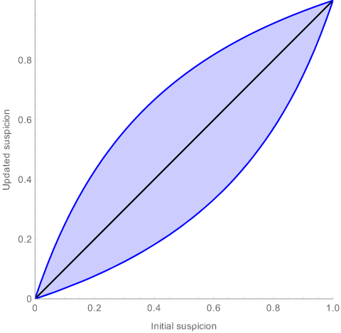
With differential privacy, the updated probability(suspicion) is never too far from the initial suspicion. The black line is what happens if the attacker didn ’ ’ ’t get their suspicion updated at all. The blue lines are the lower and upper bounds on the updated suspicion: it can be anywhere between the two.
\,
Proof :
\,
Bayes ’ ’ ’ rule : P [ D = D ∣ A ( D ) = O ] = P [ D = D ] ⋅ P [ A ( D ) = O ∣ D = D ] P [ A ( D ) = O ] \mathbb P[\mathcal D=D∣A(\mathcal D)=\mathcal O] = \frac{ \mathbb P[\mathcal D=D] · \mathbb P[A(\mathcal D)=\mathcal O∣\mathcal D=D] }{ P[A(\mathcal D)=\mathcal O] } P[D=D∣A(D)=O]=P[A(D)=O]P[D=D]⋅P[A(D)=O∣D=D]
\,
P [ D = D ∣ A ( D ) = O ] P [ D = D ′ ∣ A ( D ) = O ] = P [ D = D ] ⋅ P [ A ( D ) = O ∣ D = D ] P [ D = D ′ ] ⋅ P [ A ( D ) = O ∣ D = D ′ ] = P [ D = D ] ⋅ P [ A ( D ) = O ] P [ D = D ′ ] ⋅ P [ A ( D ′ ) = O ] \frac{ \mathbb P[\mathcal D=D∣A(\mathcal D)=\mathcal O] }{ \mathbb P[\mathcal D=D'∣A(\mathcal D)=\mathcal O] } = \frac{ \mathbb P[\mathcal D=D] · \mathbb P[A(\mathcal D)=\mathcal O∣\mathcal D=D] }{ \mathbb P[\mathcal D=D'] · \mathbb P[A(\mathcal D)=\mathcal O∣\mathcal D=D'] } = \frac{ \mathbb P[\mathcal D=D] · \mathbb P[A(D)=\mathcal O] }{ \mathbb P[\mathcal D=D'] · \mathbb P[A(D')=\mathcal O] } P[D=D′∣A(D)=O]P[D=D∣A(D)=O]=P[D=D′]⋅P[A(D)=O∣D=D′]P[D=D]⋅P[A(D)=O∣D=D]=P[D=D′]⋅P[A(D′)=O]P[D=D]⋅P[A(D)=O]
\,
Differential privacy : e − ε ≤ P [ A ( D ) = O ] P [ A ( D ′ ) = O ] ≤ e ε e^{-\varepsilon} \le \frac{ \mathbb P[A(D)=\mathcal O] }{ \mathbb P[A(D')=\mathcal O] } \le e^\varepsilon e−ε≤P[A(D′)=O]P[A(D)=O]≤eε
\,
e − ε ⋅ P [ D = D ] P [ D = D ′ ] ≤ P [ D = D ∣ A ( D ) = O ] P [ D = D ′ ∣ A ( D ) = O ] ≤ e ε ⋅ P [ D = D ] P [ D = D ′ ] e^{-\varepsilon} · \frac{\mathbb{P}\left[\mathcal D=D\right]}{\mathbb{P}\left[\mathcal D=D'\right]} \le \frac{\mathbb{P}\left[\mathcal D=D\mid A(\mathcal D)=\mathcal O\right]}{\mathbb{P}\left[\mathcal D=D'\mid A(\mathcal D)=\mathcal O\right]} \le e^\varepsilon · \frac{\mathbb{P}\left[\mathcal D=D\right]}{\mathbb{P}\left[\mathcal D=D'\right]} e−ε⋅P[D=D′]P[D=D]≤P[D=D′∣A(D)=O]P[D=D∣A(D)=O]≤eε⋅P[D=D′]P[D=D]
\,
Replace P [ D = D ′ ] \mathbb P[\mathcal D=D'] P[D=D′] with 1 − P [ D = D ] 1-\mathbb P[\mathcal D=D] 1−P[D=D], do the same for P [ D = D ′ ∣ A ( D ) = O ] \mathbb{P}\left[\mathcal D=D' | A(\mathcal D)=\mathcal O\right] P[D=D′∣A(D)=O], and solve for P [ D = D ∣ A ( D ) = O ] \mathbb{P}\left[\mathcal D=D | A(\mathcal D)=\mathcal O\right] P[D=D∣A(D)=O]
\,
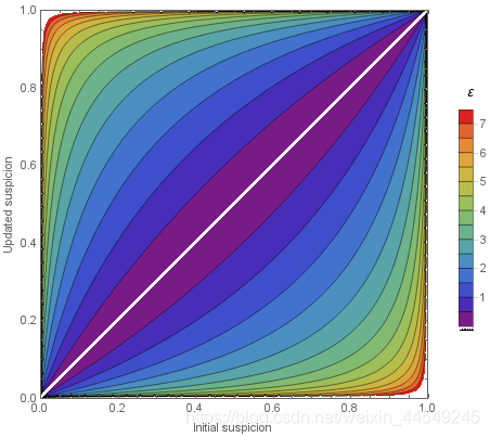
P [ D = D ] e ε + ( 1 − e ε ) ⋅ P [ D = D ] ≤ P [ D = D ∣ A ( D ) = O ] ≤ e ε ⋅ P [ D = D ] 1 + ( e ε − 1 ) ⋅ P [ D = D ] \frac{\mathbb{P}\left[\mathcal D=D\right]}{e^{\varepsilon}+\left(1-e^{\varepsilon}\right) · \mathbb{P}\left[\mathcal D=D\right]} \leq \mathbb{P}\left[\mathcal D=D\mid A\left(\mathcal D\right)=\mathcal O\right] \leq \frac{e^{\varepsilon} · \mathbb{P}\left[\mathcal D=D\right]}{1+\left(e^{\varepsilon}-1\right)\cdot\mathbb{P}\left[\mathcal D=D\right]} eε+(1−eε)⋅P[D=D]P[D=D]≤P[D=D∣A(D)=O]≤1+(eε−1)⋅P[D=D]eε⋅P[D=D]
\,
We can draw a generalization of this graph for various values of ε \varepsilon ε :
The privacy loss random variable
Recall the proof above. We saw that ε \varepsilon ε bounds the evolution of betting odds : P [ D = D 1 ∣ A ( D ) = O ] P [ D = D 2 ∣ A ( D ) = O ] ≤ e ε ⋅ P [ D = D 1 ] P [ D = D 2 ] \frac{\mathbb{P}\left[D=D_1\mid A(D)=O\right]}{\mathbb{P}\left[D=D_2\mid A(D)=O\right]} \le e^\varepsilon · \frac{\mathbb{P}\left[D=D_1\right]}{\mathbb{P}\left[D=D_2\right]} P[D=D2∣A(D)=O]P[D=D1∣A(D)=O]≤eε⋅P[D=D2]P[D=D1]
Let us define:
L D 1 , D 2 ( O ) = ln P [ D = D 1 ∣ A ( D ) = O ] P [ D = D 2 ∣ A ( D ) = O ] P [ D = D 1 ] P [ D = D 2 ] = ln ( P [ A ( D 1 ) = O ] P [ A ( D 2 ) = O ] ) \mathcal{L}_{D_1,D_2}(O) = \ln\frac{ \, \frac{ \mathbb{P}\left[D=D_1\mid A(D)=O\right]}{\mathbb{P}\left[D=D_2\mid A(D)=O\right]} \,}{ \frac{\mathbb{P}\left[D=D_1\right]}{\mathbb{P}\left[D=D_2\right]} } = \ln\left(\frac{\mathbb{P}\left[A(D_1)=O\right]}{\mathbb{P}\left[A(D_2)=O\right]}\right) LD1,D2(O)=lnP[D=D2]P[D=D1]P[D=D2∣A(D)=O]P[D=D1∣A(D)=O]=ln(P[A(D2)=O]P[A(D1)=O])
Intuitively, the privacy loss random variable is the actual ε \varepsilon ε value for a specific output O O O.
在定义 P [ A ( D 1 ) = O ] ≤ e ε ⋅ P [ A ( D 2 ) = O ] \mathbb{P}[A(D_1)=O] \le e^\varepsilon · \mathbb{P}[A(D_2)=O] P[A(D1)=O]≤eε⋅P[A(D2)=O] 中取 ≤ \le ≤的体现:
 \quad\,\,\,\,
实际上只有当输出 O O O 在 O = A ( D 1 ) O=A(D_1) O=A(D1) 与 O = A ( D 2 ) O=A(D_2) O=A(D2) 之间时才取 < < < , 此时同样 L D 1 , D 2 ( O ) ≤ ε \mathcal{L}_{D_1,D_2}(O) \le \varepsilon LD1,D2(O)≤ε 只取 < < <
δ \delta δ in ( ε , δ ) (\varepsilon,\delta) (ε,δ)- D P DP DP
δ = ∑ O P [ A ( D 1 ) = O ] ⋅ max ( 0 , 1 − e ε − L D 1 , D 2 ( O ) ) = E O ∼ A ( D 1 ) [ max ( 0 , 1 − e ε − L D 1 , D 2 ( O ) ) ] \delta \,\,\,=\,\,\, \sum_{O} \mathbb{P}[A(D_1)=O] \, · \max\left(0, 1 -e^{\varepsilon-{\mathcal{L}_{D_1,D_2}(O)}}\right) \,\,\,=\,\,\, \mathbb{E}_{O\sim A(D_1)} \left[ \max\left(0, 1 - e^{\varepsilon-{\mathcal{L}_{D_1,D_2}(O)}}\right)\right] δ=O∑P[A(D1)=O]⋅max(0,1−eε−LD1,D2(O))=EO∼A(D1)[max(0,1−eε−LD1,D2(O))]
Intuitively, in ( ε , δ ) (\varepsilon,\delta) (ε,δ)-DP, the δ \delta δ is the area highlighted below.
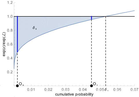
注 : 使用高斯噪声时, 若仅仅直观地将 δ \,\delta\, δ理解为是 ( ε , 0 ) \,(\varepsilon,0) (ε,0)- D P DP\, DP即传统 ε \,\varepsilon ε- D P DP\, DP的定义可以被违反的概率, 则是选取了 δ = δ 1 \,\delta=\delta_1 δ=δ1
但实际上 δ 2 \,\delta_2 δ2更紧。从上图可见 , δ 2 < δ 1 \delta_2<\delta_1 δ2<δ1 , 因为 δ 1 \,\delta_1 δ1在上图中也可以看作是长为 δ 1 \,\delta_1 δ1宽为1的矩形面积, 显然大于阴影部分的面积 δ 2 \,\delta_2 δ2
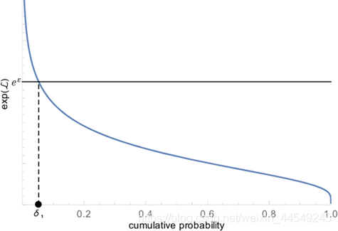
上述 δ 1 \,\delta_1\, δ1( \, 即传统 ε \,\varepsilon ε- D P DP\, DP的定义可以被违反的概率 \, ) \, 的直观意义如下图 :
Proof :
\,
The definition of ( ε , δ ) (\varepsilon,\delta) (ε,δ)- D P DP DP : P [ A ( D 1 ) ∈ S ] ≤ e ε ⋅ P [ A ( D 2 ) ∈ S ] + δ . \mathbb{P}[A(D_1)\in S] \le e^\varepsilon\cdot\mathbb{P}[A(D_2)\in S]+\delta. P[A(D1)∈S]≤eε⋅P[A(D2)∈S]+δ.
Fix a mechanism A A A and a ε ≥ 0 \varepsilon \ge0 ε≥0. For each possible set of outputs S S S, we can compute:
\,
δ = max S ( P [ A ( D 1 ) ∈ S ] − e ε ⋅ P [ A ( D 2 ) ∈ S ] ) \delta = \max_{S} \left(\mathbb{P}[A(D_1)\in S] - e^\varepsilon\cdot\mathbb{P}[A(D_2)\in S]\right) δ=maxS(P[A(D1)∈S]−eε⋅P[A(D2)∈S])
\,
The set S S S that maximizes the quantity above is:
\,
S m a x = { O ∣ P [ A ( D 1 ) = O ] > e ε ⋅ P [ A ( D 2 ) = O ] } = { O ∣ L D 1 , D 2 ( O ) > ε } S_{max} = \left\{O \mid \mathbb{P}[A(D_1)=O] > e^\varepsilon\cdot\mathbb{P}[A(D_2)=O]\right\} =\{ O \mid \, \mathcal{L}_{D_1,D_2}(O)>\varepsilon \,\, \} Smax={O∣P[A(D1)=O]>eε⋅P[A(D2)=O]}={O∣LD1,D2(O)>ε}
\,
So we have:
\,
δ = P [ A ( D 1 ) ∈ S m a x ] − e ε ⋅ P [ A ( D 2 ) ∈ S m a x ] = ∑ O ∈ S m a x P [ A ( D 1 ) = O ] − e ε ⋅ P [ A ( D 2 ) = O ] = ∑ O ∈ S m a x P [ A ( D 1 ) = O ] ( 1 − e ε e L D 1 , D 2 ( O ) ) \delta = \mathbb{P}[A(D_1)\in S_{max}] - e^\varepsilon\cdot\mathbb{P}[A(D_2)\in S_{max}] \\ \,\,\,\,\, = \sum_{O\in S_{max}} \mathbb{P}[A(D_1)=O] - e^\varepsilon\cdot\mathbb{P}[A(D_2)=O] \\ \,\,\,\,\, = \sum_{O\in S_{max}} \mathbb{P}[A(D_1)=O] \left(1 - \frac{e^\varepsilon}{e^{\mathcal{L}_{D_1,D_2}(O)}}\right) δ=P[A(D1)∈Smax]−eε⋅P[A(D2)∈Smax]=∑O∈SmaxP[A(D1)=O]−eε⋅P[A(D2)=O]=∑O∈SmaxP[A(D1)=O](1−eLD1,D2(O)eε)
\,
δ = ∑ O P [ A ( D 1 ) = O ] ⋅ max ( 0 , 1 − e ε − L D 1 , D 2 ( O ) ) = E O ∼ A ( D 1 ) [ max ( 0 , 1 − e ε − L D 1 , D 2 ( O ) ) ] \delta = \sum_{O} \mathbb{P}[A(D_1)=O] \, · \max\left(0, 1 -e^{\varepsilon-{\mathcal{L}_{D_1,D_2}(O)}}\right) \,\,\,=\,\,\, \mathbb{E}_{O\sim A(D_1)} \left[ \max\left(0, 1 - e^{\varepsilon-{\mathcal{L}_{D_1,D_2}(O)}}\right)\right] δ=∑OP[A(D1)=O]⋅max(0,1−eε−LD1,D2(O))=EO∼A(D1)[max(0,1−eε−LD1,D2(O))]
Composition
C C C is the algorithm which combines A A A and B B B : C ( D ) = ( A ( D ) , B ( D ) ) C( \mathcal D )=( A(\mathcal D) , B(\mathcal D)) C(D)=(A(D),B(D)).
The output of this algorithm will be a pair of outputs: O = ( O A , O B ) \mathcal O=(\mathcal O_A , \mathcal O_B) O=(OA,OB).
C C C is ( ε A \varepsilon_A εA+ ε B \varepsilon_B εB)-differentially private. / C C C is ( ε A \varepsilon_A εA+ ε B \varepsilon_B εB , δ A \delta_A δA+ δ B \delta_B δB)-differentially private.
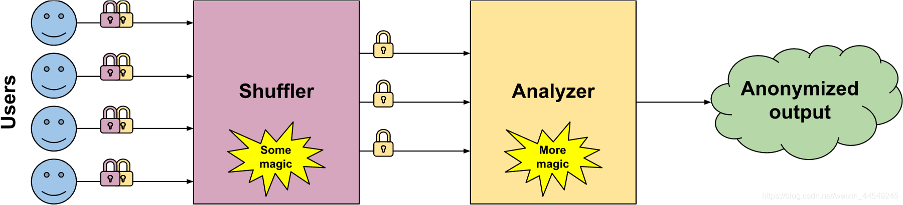
ESA (Encode, Shuffle, Analyze) The best of both worlds (Local vs. Global differential privacy).
Until very recently, there was no middle ground between the two options. The choice was binary: either accept a much larger level of noise (Local differential privacy), or collect raw data (Global differential privacy). This is starting to change, thanks to recent work on a novel type of architecture called ESA.
- The encoder is a fancy name to say “user”. It collects the data, encrypts it twice in two layers, and passes it to the shuffler.
- The shuffler can only decrypt the first layer. It contains the user IDs, and something called “group ID”. This group ID describes what kind of data this is, but not what is the actual value of the data. First, The shuffler removes identifiers, and groups all group IDs together and counts how many users are in each group. Then, it passes them all to the analyzer if there are enough of them.
- The analyzer can then decrypt the second layer of the data, and compute the output.
eee
Ref
博文参考链接(Google)
博文参考链接(DP创始者之一)
这篇关于【基础储备】Differential Privacy 基础知识储备的文章就介绍到这儿,希望我们推荐的文章对编程师们有所帮助!


