本文主要是介绍【论文研读】Online Advertisement Allocation in the Presence of Customer Choices-1,希望对大家解决编程问题提供一定的参考价值,需要的开发者们随着小编来一起学习吧!
【论文研读】Online Advertisement Allocation in the Presence of Customer Choices-1
- 背景介绍
- 专有名词
- 摘要
- 问题描述
- 参数
- 模型假设
- 数学模型
- 两阶段随机优化模型
- 第一阶段
- 第二阶段
- 证明两阶段随机规划模型的最优性
- 最优性证明
- 参考文献
背景介绍
近10年来,互联网技术和智能手机普及率快速增长,网络广告成为空前庞大的产业,对整个经济产生重大影响。美国互动广告局报告称,2019 年美国市场在线广告收入增至 1246 亿美元(同比增长率为 16%,自 2010 年以来年均增长率为 19%)。事实上,Facebook 等大型在线平台将其大规模用户流量变现的主要方式是在线广告。例如,2019 年,Facebook 从广告中获得了 697 亿美元的收入,占其总收入的 98.53%2
专有名词
- CPC(cost-per-click):客户点击广告时,广告商向平台支付的费用。(advertisers pay an advertising fee to the platform when customers click their ads)
- 广告计划是提前制定的:电子商务平台要求广告商每天提交他们的广告计划,指定一天中显示广告的时间间隔(小时),以及相应的每次点击费用。
- click-through (lower-limit) constraint :电商平台从商家获取收益的客户点击量要求,即推广的广告达到被点击的最少次数,电商平台才能获得收益
- organic recommendations:“有机推荐"或者"自然推荐”,通常指的是人们在互联网上的搜索过程中,基于一些算法和数据分析,由搜索引擎或其他相关平台为用户提供与其搜索词相关且有机的、非付费的推荐结果。相对于付费广告推荐,“organic recommendations” 更侧重于提供有价值、可信度更高的有效信息给用户。
- cannibalization:“市场份额蚕食”或“内部竞争”
- UVs:user views,用户画像,与可能成为潜在买家的商家匹配
摘要
要点提取:
- 视角:电子商务平台运营商
- 目标:最大化规定周期内的广告收益
- 必要性:广告的点击量对广告主的长期留存有实质性影响,促使平台设计广告分配策略以确保一定的点击量
- 方法:two stage stochastic program
-
- 一阶段:匹配广告/客户类型
-
- 二阶段:设计广告分配策略
- 最优性证明:
-
- 1.reduce to a scalable linear program if the customer click-through behavior follows the multinomial logit model
-
- 2.provide a family of debt-weighted algorithms to achieve the optimal click-through goals, and prove that they are asymptotically optimal when the problem size scales to infinity
问题描述
如何将每个时段内的广告集合内的部分广告推送给潜在的客户便是一个中央运营问题(central operations problem),即动态选择一组广告(商家提供的广告计划,包括展示的时间段和报价)推荐给每个到达的客户,以便在整个规划范围内产生最高的总价值。这里平台对于广告集合的大小需要做出一个决策,即权衡广告集合的大小,既要保证平台的广告收益所以需要扩大广告集合,但也需要减小同类商家广告的竞争,所以需要控制广告集的大小。并且不同广告的潜在客户的活跃时间段的不同以及最低点击量的要求,也需要平台做出更好的推荐方案。
在制定平台的广告投放计划时,还需要考虑以下的约束:
- 商家的潜在客户的活跃时间段不同
- 广告商投放广告的预算是有限的
- 广告的最低点击量要求
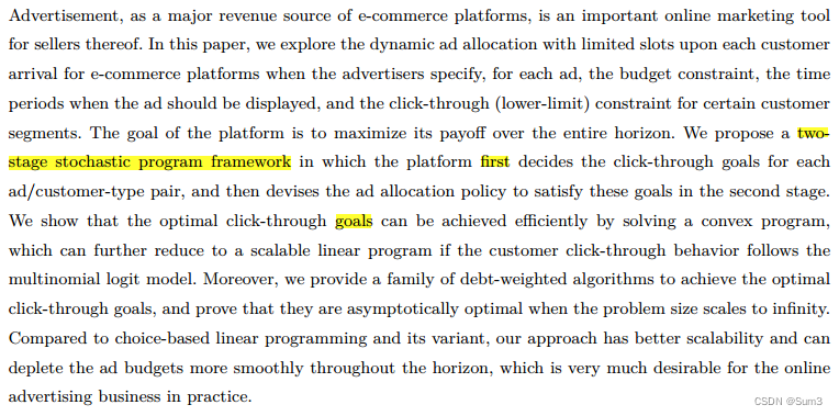
如图所示,不同的商家(Campaign)向平台提交自己的广告投放计划,然后当某位用户访问平台的时候,首先从在该周期内有广告计划的商家与用户匹配,将配对成功的商家的广告为其投放,然后如果用户点击了广告并且商家的最低点击量要求满足,就会消耗商家为该广告的投入预算,即平台会开始向商家收取费用。
z = min x , s , y ∑ i , j ∈ N ∪ { 0 } x i j t i j ( 1 ) s . t . ∑ i ∈ N c ∑ j ∈ N ∪ { 0 } / { i } x i j = 1 , ∀ c ∈ C , ( 2 ) ∑ j ∈ N ∪ { 0 } / { i } x i j = ∑ j ∈ N ∪ { 0 } / { i } x j i , ∀ i ∈ N ∪ { 0 } , ( 3 ) ∑ i ∈ N x 0 i ⩽ ∣ V ∣ , ( 4 ) ∑ i ∈ N c a i c ∑ j ∈ N ∪ { 0 } / { i } x i j ⩽ s c ⩽ ∑ i ∈ N c b i c ∑ j ∈ N ∪ { 0 } / { i } x i j , ∀ c ∈ C , ( 5 ) s c + ∑ i ∈ N c ∑ j ∈ N c ′ t i j x i j ⩽ s c ′ + T ( 1 − ∑ i ∈ N c ∑ j ∈ N c ′ x i j ) , ∀ c ∈ C ∪ { 0 } , c ′ ∈ C / { c } , ( 6 ) 0 ⩽ y c ⩽ Q − d c , ∀ c ∈ C , ( 7 ) y c + Q ( 1 − ∑ i ∈ N c ∑ j ∈ N c ′ x i j ) ⩾ d c ′ + y c ′ , ∀ c ∈ C ∪ { 0 } , c ′ ∈ C / { c } , ( 8 ) x i j ∈ { 0 , 1 } , ∀ i , j ∈ N ∪ { 0 } . ( 9 ) \begin{aligned} z = \min\limits_{x,s,y} &\sum\limits_{i,j \in N \cup \{0\}} x_{ij}t_{ij} &&\quad \quad (1) \\ s.t. &\sum \limits_ {i \in N_c}\sum\limits_{j \in N \cup \{0\} / \{i\}} x_{ij}=1, \quad &&\forall c\in C, \quad \quad (2) \\ &\sum\limits_{j \in N \cup \{0\} / \{i\}} x_{ij}=\sum\limits_{j \in N \cup \{0\} / \{i\}} x_{ji}, \quad &&\forall i \in N \cup \{0\}, \quad \quad (3) \\ &\sum \limits_ {i \in N} x_{0i} \leqslant |V|, &&\quad \quad (4) \\ &\sum \limits_ {i \in N_c} a_i^c\sum\limits_{j \in N \cup \{0\} / \{i\}} x_{ij} \leqslant s_c \leqslant \sum \limits_ {i \in N_c} b_i^c\sum\limits_{j \in N \cup \{0\} / \{i\}} x_{ij}, \quad &&\forall c \in C, \quad \quad (5) \\ &s_c+\sum \limits_ {i \in N_c}\sum \limits_ {j \in N_{c'}}t_{ij}x_{ij} \leqslant s_{c'}+T(1-\sum \limits_ {i \in N_c}\sum \limits_ {j \in N_{c'}}x_{ij}), \quad &&\forall c \in C \cup\{0\}, {c'} \in C/\{c\}, \quad \quad (6) \\ &0 \leqslant y_c \leqslant Q-d_c, \quad &&\forall c \in C, \quad \quad (7) \\ &y_c +Q(1-\sum \limits_ {i \in N_c}\sum \limits_ {j \in N_{c'}}x_{ij}) \geqslant d_{c'}+y_{c'}, \quad &&\forall c \in C \cup \{0\}, {c'} \in C/\{c\}, \quad \quad (8) \\ &x_{ij} \in \{0,1\}, \quad &&\forall i,j \in N \cup \{0\}. \quad \quad (9) \end{aligned} z=x,s,ymins.t.i,j∈N∪{0}∑xijtiji∈Nc∑j∈N∪{0}/{i}∑xij=1,j∈N∪{0}/{i}∑xij=j∈N∪{0}/{i}∑xji,i∈N∑x0i⩽∣V∣,i∈Nc∑aicj∈N∪{0}/{i}∑xij⩽sc⩽i∈Nc∑bicj∈N∪{0}/{i}∑xij,sc+i∈Nc∑j∈Nc′∑tijxij⩽sc′+T(1−i∈Nc∑j∈Nc′∑xij),0⩽yc⩽Q−dc,yc+Q(1−i∈Nc∑j∈Nc′∑xij)⩾dc′+yc′,xij∈{0,1},(1)∀c∈C,(2)∀i∈N∪{0},(3)(4)∀c∈C,(5)∀c∈C∪{0},c′∈C/{c},(6)∀c∈C,(7)∀c∈C∪{0},c′∈C/{c},(8)∀i,j∈N∪{0}.(9)
参数
| 符号 | 含义 |
|---|---|
| ∑ \sum ∑ | 一个广告推荐计划的时间范围为一天,由 ∑ \sum ∑个周期组成,即 { 1 , 2 , … , ∑ } \{1,2,\dots,\sum\} {1,2,…,∑} |
| s s s | 表示第 s s s个周期 |
| T T T | 一天内访问平台的客户总数 |
| ζ s \zeta_s ζs | 表示周期 s s s内访问的客户占比,即 T s = ζ s T T_s=\zeta_sT Ts=ζsT, ∑ s = 1 ∑ ζ s = 1 \sum_{s=1}^{\sum}\zeta_s=1 ∑s=1∑ζs=1 |
| N \mathcal{N} N | 广告集合 N : = { 1 , 2 , … , n } \mathcal{N}:=\{1,2,\dots,n\} N:={1,2,…,n},用 0 0 0表示有机推荐,所以有 N ˉ = N ∪ { 0 } \bar{\mathcal{N}}=\mathcal{N}\cup\{0\} Nˉ=N∪{0} |
| ∣ N s ∣ |\mathcal{N}_s| ∣Ns∣ | 表示周期 s s s内的活跃广告集合 n s : = ∣ N s ∣ n_s:=|\mathcal{N}_s| ns:=∣Ns∣,对于每个周期 s s s内则有 N s ˉ = N s ∪ { 0 } \bar{\mathcal{N}_s}=\mathcal{N}_s\cup\{0\} Nsˉ=Ns∪{0} |
| σ \sigma σ | 某商家广告开始的周期 |
| K K K | 某商家广告持续的周期数 |
| B B B | 某商家广告投入的总预算,向平台支付的最大广告费金额, B > 0 B>0 B>0 |
| b b b | 某商家为广告的单次点击支付的费用, b > 0 b>0 b>0 |
| λ \lambda λ | 商家的参数向量, λ i = ( σ i , K i , B i , b i ) , i ∈ N \lambda_i=(\sigma_i,K_i,B_i,b_i),i\in\mathcal{N} λi=(σi,Ki,Bi,bi),i∈N |
| S s t S_s^t Sst | 向在周期 s s s访问平台的用户 t t t可能展示的广告集合(与之配对的商家的广告), S s t ∈ N s S_s^t\in \mathcal{N}_s Sst∈Ns |
| S j \mathcal{S_j} Sj | 类型为 j j j的用户的所有可能的广告集合的集合 |
| r i r_i ri | 某商家为广告 i i i的单次点击的价值, i ∈ N ˉ i\in\bar{\mathcal{N}} i∈Nˉ,有机推荐的价值 r 0 r_0 r0一般比普通的 r i r_i ri低一个数量级。 |
特别的在有机推荐中,广告商不向平台付费,文中假设 B 0 = + ∞ B_0=+\infty B0=+∞, b 0 = 0 b_0=0 b0=0, σ 0 = 1 \sigma_0=1 σ0=1, K 0 = ∑ K_0=\sum K0=∑。
模型假设
首先假设在某个周期 s s s内访问平台的客户 T s T_s Ts是按照时间顺序访问的,有 T s = { 1 , 2 , … , T s } \mathcal{T}_s=\{1,2,\dots,T_s\} Ts={1,2,…,Ts}。对于在该周期每个访问平台的客户 t t t的用户类型 ξ s t \xi_{\mathcal{s}}^t ξst(可以理解为用户画像,即会与商家有匹配的情况)是独立分布的,并且遵循在 M \mathcal{M} M的离散分布,即 P ( ξ s t = j ) = p j s , j ∈ M \mathbb{P}(\xi_s^t=j)=p_j^s,j\in\mathcal{M} P(ξst=j)=pjs,j∈M,所以有 ∑ j ∈ M p j s = 1 \sum_{j\in\mathcal{M}}p_j^s=1 ∑j∈Mpjs=1。
于是设决策变量如下
| 符号 | 含义 |
|---|---|
| y i j ( S ) y_i^j(S) yij(S) | 当广告集 S S S时,类型为 j j j的客户在广告 i i i上的点击总数, y i j ( S ) ∈ Z + y_i^j(S)\in\mathbb{Z}^+ yij(S)∈Z+, i ∈ S , j ∈ M i\in S,j\in \mathcal{M} i∈S,j∈M |
| ϕ i j ( S ) \phi_i^j(S) ϕij(S) | 当广告集 S S S时,类型为 j j j的客户在广告 i i i上的期望点击数, ϕ i j ( S ) : = E [ y i j ( S ) ] \phi_i^j(S):=\mathbb{E}[y_i^j(S)] ϕij(S):=E[yij(S)], ϕ i j ( S ) < + ∞ \phi_i^j(S)<+\infty ϕij(S)<+∞, i ∈ S , j ∈ M i\in S,j\in \mathcal{M} i∈S,j∈M,如果 i ∉ S i \notin S i∈/S, y i j ( S ) = 0 , ϕ i j ( S ) = 0 y_i^j(S)=0,\phi_i^j(S)=0 yij(S)=0,ϕij(S)=0 |
从商家的角度来看,他们根据客户过去的行为模式、潜在的兴趣和人口统计学信息,将广告定位到相关的客户群。例如,商家可能要求平台将其尿布广告定位到新父母。所以每个广告 i ∈ N i\in \mathcal{N} i∈N以潜在的客户群体 L i ⊆ M \mathcal{L}_i\subseteq\mathcal{M} Li⊆M为特征(target)进行分类。对于有机推荐,平台不会对其可能展示的客户群体施加限制,即 L 0 = M \mathcal{L}_0=\mathcal{M} L0=M。另外设 η i c \eta_i^c ηic为广告 i i i在一天内被客户 c ⊆ L i c \subseteq \mathcal{L}_i c⊆Li的最小点击数,那么对于有机推荐有 η 0 c = 0 \eta_0^c=0 η0c=0, c ∈ M c\in \mathcal{M} c∈M。同样的也存在有的商家不会给平台设置最低的点击量要求,那么就可以设其 η i c = 0 \eta_i^c=0 ηic=0。
∑ s = σ i σ i + K i − 1 ∑ t = 1 T s ∑ j ∈ c y i j ( S s t ) 1 { ξ s t = j } ⩾ η i c i ∈ N , c ⊆ L i \begin{aligned} \sum_{s=\sigma_i}^{\sigma_i+K_i-1}\sum_{t=1}^{T_s}\sum_{j\in c}y_i^j(S_{\mathcal{s}}^t)1_{\{\xi_s^t=j\}}\geqslant \eta_i^c \quad \quad i\in \mathcal{N},c\subseteq \mathcal{L}_i \end{aligned} s=σi∑σi+Ki−1t=1∑Tsj∈c∑yij(Sst)1{ξst=j}⩾ηici∈N,c⊆Li
在周期 s s s内访问平台的一个用户 ξ s t = j \xi_s^t=j ξst=j,平台可以向其展示的广告集合 S s t ∈ S i ⊂ 2 N s S_s^t\in \mathcal{S}_i\subset2^{\mathcal{N}_s} Sst∈Si⊂2Ns,其中 2 N s 2^{\mathcal{N}_s} 2Ns为 N s {\mathcal{N}_s} Ns的幂集。也就是说如果当 ξ s t = j \xi_s^t=j ξst=j,对于任何的广告 i ∈ S s t ∈ S j i\in S_s^t \in\mathcal{S}_j i∈Sst∈Sj都有 j ∈ L i j\in \mathcal{L}_i j∈Li,换言之任何类型的用户都必须在向其展示的广告的目标集中。
数学模型
将平台的广告分配问题描述为一个多周期随机规划。具体地说,该平台寻求优化全天的总预期价值:
max E [ ∑ s = 1 ∑ ∑ t = 1 T s ∑ i ∈ N s r i y i ξ s t ( S s t ) ] ( 1.1 ) s . t . ∑ s = σ i σ i + K i − 1 ∑ t = 1 T s b i y i ξ i t ( S s t ) ⩽ B i , a l m o s t s u r e l y f o r e a c h i ∈ N , ( 1.2 ) ∑ s = σ i σ i + K i − 1 ∑ t = 1 T s ∑ j ∈ c y i j ( S s t ) 1 { ξ s t = j } ⩾ η i c , a l m o s t s u r e l y f o r e a c h i ∈ N a n d c ⊆ L i , ( 1.3 ) 0 ∈ S s t ⊆ N s ˉ f o r e a c h s , t . \begin{aligned} & \max && \mathbb{E} \left [ \sum_{s=1}^{\sum}\sum_{t=1}^{T_s}\sum_{i \in \mathcal{N}_s} r_iy_i^{\xi_s^t}(S_{\mathcal{s}}^t) \right ] &(1.1) \\ & s.t. && \sum_{s=\sigma_i}^{\sigma_i+K_i-1}\sum_{t=1}^{T_s}b_iy_i^{\xi_i^{t}}(S_{\mathcal{s}}^t) \leqslant B_i ,almost \quad surely \quad for \quad each \quad i \in N , &(1.2) \\ & && \sum_{s=\sigma_i}^{\sigma_i+K_i-1}\sum_{t=1}^{T_s}\sum_{j\in c}y_i^j(S_{\mathcal{s}}^t)1_{\{\xi_s^t=j\}}\geqslant \eta_i^c ,almost \quad surely \quad for \quad each \quad i \in \mathcal{N} and c \subseteq \mathcal{L}_i , &(1.3) \\ & && 0\in S_{\mathcal{s}}^t \subseteq \bar{\mathcal{N}_s} \quad for \quad each \quad s,t. \end{aligned} maxs.t.E s=1∑∑t=1∑Tsi∈Ns∑riyiξst(Sst) s=σi∑σi+Ki−1t=1∑Tsbiyiξit(Sst)⩽Bi,almostsurelyforeachi∈N,s=σi∑σi+Ki−1t=1∑Tsj∈c∑yij(Sst)1{ξst=j}⩾ηic,almostsurelyforeachi∈Nandc⊆Li,0∈Sst⊆Nsˉforeachs,t.(1.1)(1.2)(1.3)
约束 ( 1.2 ) (1.2) (1.2)是每个广告的预算约束,约束 ( 1.3 ) (1.3) (1.3)是每个广告相对于不同客户集合的最低点击量要求。
最大化每个客户价值的数学模型
max E [ 1 T ∑ s = 1 ∑ ∑ t = 1 T s ∑ i ∈ N s r i y i ξ s t ( S s t ) ] ( 2.1 ) s . t . 1 T ( i ) ∑ s = σ i σ i + K i − 1 ∑ t = 1 T s b i y i ξ i t ( S s t ) ⩽ B i T ( i ) , a l m o s t s u r e l y f o r e a c h i ∈ N , ( 2.2 ) 1 T ( i ) ∑ s = σ i σ i + K i − 1 ∑ t = 1 T s ∑ j ∈ c y i j ( S s t ) 1 { ξ s t = j } ⩾ η i c T ( i ) , a l m o s t s u r e l y f o r e a c h i ∈ N a n d c ⊆ L i , ( 2.3 ) 0 ∈ S s t ⊆ N s ˉ f o r e a c h s , t . \begin{aligned} & \max && \mathbb{E} \left [ \frac{1}{T}\sum_{s=1}^{\sum}\sum_{t=1}^{T_s}\sum_{i \in \mathcal{N}_s} r_iy_i^{\xi_s^t}(S_{\mathcal{s}}^t) \right ] &(2.1) \\ & s.t. && \frac{1}{T(i)} \sum_{s=\sigma_i}^{\sigma_i+K_i-1}\sum_{t=1}^{T_s}b_iy_i^{\xi_i^{t}}(S_{\mathcal{s}}^t) \leqslant \frac{B_i}{T(i)} ,almost \quad surely \quad for \quad each \quad i \in N , &(2.2) \\ & && \frac{1}{T(i)}\sum_{s=\sigma_i}^{\sigma_i+K_i-1}\sum_{t=1}^{T_s}\sum_{j\in c}y_i^j(S_{\mathcal{s}}^t)1_{\{\xi_s^t=j\}}\geqslant \frac{\eta_i^c}{T(i)} ,almost \quad surely \quad for \quad each \quad i \in \mathcal{N} and c \subseteq \mathcal{L}_i , &(2.3) \\ & && 0\in S_{\mathcal{s}}^t \subseteq \bar{\mathcal{N}_s} \quad for \quad each \quad s,t. \end{aligned} maxs.t.E T1s=1∑∑t=1∑Tsi∈Ns∑riyiξst(Sst) T(i)1s=σi∑σi+Ki−1t=1∑Tsbiyiξit(Sst)⩽T(i)Bi,almostsurelyforeachi∈N,T(i)1s=σi∑σi+Ki−1t=1∑Tsj∈c∑yij(Sst)1{ξst=j}⩾T(i)ηic,almostsurelyforeachi∈Nandc⊆Li,0∈Sst⊆Nsˉforeachs,t.(2.1)(2.2)(2.3)
其中
T ( i ) : = ∑ s = σ i σ i + K i − 1 T s , i ∈ N \begin{aligned} T(i):=\sum_{s=\sigma_i}^{\sigma_i+K_i-1}T_s, \quad i \in \mathcal{N} \end{aligned} T(i):=s=σi∑σi+Ki−1Ts,i∈N
为了简化上面的模型 ( 2 ) (2) (2),引入了一个辅助决策变量 α = ( α i j ( s ) ⩾ 0 : i ∈ N ˉ , j ∈ M , 1 ⩽ s ⩽ ∑ ) \alpha=(\alpha_i^j(s)\geqslant0:i\in \bar{\mathcal{N}},j\in \mathcal{M}, 1\leqslant s \leqslant \sum) α=(αij(s)⩾0:i∈Nˉ,j∈M,1⩽s⩽∑)来表示周期 s s s内来自客户类型 j j j的单个客户对广告 i i i的每个用户点击次数。因此只有当满足 j ∈ L i j\in\mathcal{L}_i j∈Li与 σ i ⩽ s ⩽ σ i + K i − 1 \sigma_i\leqslant s \leqslant \sigma_i+K_i-1 σi⩽s⩽σi+Ki−1时才有 α i j ( s ) > 0 \alpha_i^j(s)>0 αij(s)>0。换言之,只有当某位用户访问时,在该周期有与之配对的商家投放的广告计划,才会有点击量。于是把模型 ( 2 ) (2) (2)可以等价写成下面的形式
max α ∑ s = 1 ∑ ζ s ∑ i ∈ N ˉ r i ∑ j ∈ L i α i j ( s ) ( 3.1 ) s . t . 1 T s ∑ t = 1 T s y i j ( S s t ) 1 { ξ s t = j } ⩾ α i j ( s ) , a l m o s t s u r e l y f o r e a c h i ∈ N ˉ , j ∈ M , s , ( 3.2 ) ∑ s = σ i σ i + K i − 1 ζ s ∑ j ∈ L i α i j ( s ) ⩽ B i T b i , ∀ i ∈ N , ( 3.3 ) ∑ s = σ i σ i + K i − 1 ζ s ∑ j ∈ L i α i j ( s ) ⩾ η i c T , ∀ i ∈ N , c ⊆ L i , ( 3.4 ) \begin{aligned} & \max_{\alpha} && \sum_{s=1}^{\sum}\zeta_s \sum_{i \in \bar {\mathcal{N}}}r_i\sum_{j\in \mathcal{L}_i}\alpha_i^j(s) &(3.1) \\ & s.t. && \frac{1}{T_s} \sum_{t=1}^{T_s}y_i^j(S_s^t)1_{\{ \xi_s^t=j \}}\geqslant\alpha_i^j(s) , almost \quad surely \quad for \quad each \quad i\in\bar{\mathcal{N}},j\in \mathcal{M},s, &(3.2) \\ & &&\sum_{s=\sigma_i}^{\sigma_i+K_i-1}\zeta_s\sum_{j\in\mathcal{L_i}} \alpha_i^j(s) \leqslant \frac{B_i}{Tb_i}, \forall i\in \mathcal{N}, &(3.3) \\ & && \sum_{s=\sigma_i}^{\sigma_i+K_i-1}\zeta_s\sum_{j\in\mathcal{L_i}} \alpha_i^j(s) \geqslant \frac{\eta_i^c}{T}, \forall i\in \mathcal{N},c\subseteq \mathcal{L_i}, &(3.4) \\ \end{aligned} αmaxs.t.s=1∑∑ζsi∈Nˉ∑rij∈Li∑αij(s)Ts1t=1∑Tsyij(Sst)1{ξst=j}⩾αij(s),almostsurelyforeachi∈Nˉ,j∈M,s,s=σi∑σi+Ki−1ζsj∈Li∑αij(s)⩽TbiBi,∀i∈N,s=σi∑σi+Ki−1ζsj∈Li∑αij(s)⩾Tηic,∀i∈N,c⊆Li,(3.1)(3.2)(3.3)(3.4)
在上式中的 1 { ⋅ } 1_{\{ \cdot \}} 1{⋅}是指示函数(Indicator function),也叫做特征函数、示性函数等。在数学上,当某个条件成立时,指示函数取值为1,否则取值为0。例如,一个实数 x x x是否属于一个集合 A A A,我们可以定义一个指示函数 I ( x ) I(x) I(x),当 x ∈ A x\in A x∈A时取值为1,否则取值为0。其表达式可以表示为:
I ( x ) = { 1 , if x ∈ A 0 , otherwise \begin{aligned} I(x) = \begin{cases} 1, & \text{if}\ x \in A \\ 0, & \text{otherwise} \end{cases} \end{aligned} I(x)={1,0,if x∈Aotherwise
两阶段随机优化模型
通过将模型 ( 3 ) (3) (3)中的约束 ( 3.2 ) (3.2) (3.2)替换为对预期点击量的约束,将 ( 3 ) (3) (3)放宽为一个两阶段的随机优化模型。在第一阶段平台做出点击量的决策 α \alpha α,然后在第二阶段从所有可能的广告推送策略中筛选出最好的决策。具体的用 G ~ \tilde{G} G~表示一个随机的广告展示策略,将用户的类型 ξ s t \xi_s^t ξst映射到广告集合中,即 S s t = S s ( ξ s t ∣ G ~ ) S_s^t=S_s(\xi_s^t|\tilde{G}) Sst=Ss(ξst∣G~)。所有可行的广告推送策略用 g ~ \tilde{\mathfrak{g}} g~表示,然后因为周期是一个离散的分布,所以有 G ~ = ( G ~ 1 , G ~ 2 , … , G ~ ∑ ) \tilde{G}=(\tilde{G}_1,\tilde{G}_2,\dots,\tilde{G}_{\sum}) G~=(G~1,G~2,…,G~∑)和 S s ( ξ s t ∣ G ~ s ) : = S s ( ξ s t ∣ G ~ ) S_s(\xi_s^t|\tilde{G}_s):=S_s(\xi_s^t|\tilde{G}) Ss(ξst∣G~s):=Ss(ξst∣G~),在某个周期 s s s中有 G ~ s ∈ g ~ s \tilde{G}_s\in\tilde{\mathfrak{g}}_s G~s∈g~s。
把模型 ( 3 ) (3) (3)的两阶段随机规划的reformulation如下
max G ~ , α ∑ s = 1 ∑ ζ s ∑ i ∈ N ˉ r i ∑ j ∈ L i α i j ( s ) ( 4.1 ) s . t . E [ y i j ( S s t ( ξ s ∣ G ~ s ) ) 1 { ξ s = j } ] ⩾ α i j ( s ) , a l m o s t s u r e l y f o r e a c h i ∈ N ˉ , j ∈ M , s , ( 4.2 ) ∑ s = σ i σ i + K i − 1 ζ s ∑ j ∈ L i α i j ( s ) ⩽ B i T b i , ∀ i ∈ N , ( 4.3 ) ∑ s = σ i σ i + K i − 1 ζ s ∑ j ∈ L i α i j ( s ) ⩾ η i c T , ∀ i ∈ N , c ⊆ L i ( 4.4 ) G ~ s ∈ g ~ s , ∀ s , \begin{aligned} & \max_{\tilde{G},\alpha} && \sum_{s=1}^{\sum}\zeta_s \sum_{i \in \bar {\mathcal{N}}}r_i\sum_{j\in \mathcal{L}_i}\alpha_i^j(s) &(4.1) \\ & s.t. && \mathbb{E}[y_i^j(S_s^t(\xi_s|\tilde{G}_s))1_{\{ \xi_s=j \}}] \geqslant\alpha_i^j(s) , almost \quad surely \quad for \quad each \quad i\in\bar{\mathcal{N}},j\in \mathcal{M},s, &(4.2) \\ & &&\sum_{s=\sigma_i}^{\sigma_i+K_i-1}\zeta_s\sum_{j\in\mathcal{L_i}} \alpha_i^j(s) \leqslant \frac{B_i}{Tb_i}, \forall i\in \mathcal{N}, &(4.3) \\ & && \sum_{s=\sigma_i}^{\sigma_i+K_i-1}\zeta_s\sum_{j\in\mathcal{L_i}} \alpha_i^j(s) \geqslant \frac{\eta_i^c}{T}, \forall i\in \mathcal{N},c\subseteq \mathcal{L_i} &(4.4) \\ & && \tilde{G}_s\in \tilde{\mathfrak{g}}_s, \forall s, \end{aligned} G~,αmaxs.t.s=1∑∑ζsi∈Nˉ∑rij∈Li∑αij(s)E[yij(Sst(ξs∣G~s))1{ξs=j}]⩾αij(s),almostsurelyforeachi∈Nˉ,j∈M,s,s=σi∑σi+Ki−1ζsj∈Li∑αij(s)⩽TbiBi,∀i∈N,s=σi∑σi+Ki−1ζsj∈Li∑αij(s)⩾Tηic,∀i∈N,c⊆LiG~s∈g~s,∀s,(4.1)(4.2)(4.3)(4.4)
其中 ξ s \xi_s ξs与 ξ s t \xi_s^t ξst的分布是相同的,其期望是关于 ξ s \xi_s ξs、 G ~ s \tilde{G}_s G~s与 y i j ( S ) y_i^j(S) yij(S)的联合分布。
第一阶段
在上面的两阶段随机规划模型 ( 4 ) (4) (4)中,第一阶段中,平台知道用户的类型的分布情况 P \mathcal{P} P和点击量的期望 Φ : = { ϕ i j ( S ) : j ∈ M , i ∈ S ⊂ N ˉ } \Phi:=\{ \phi_i^j(S):j\in \mathcal{M} ,i\in S \subset \bar{\mathcal{N}}\} Φ:={ϕij(S):j∈M,i∈S⊂Nˉ},但是不知道在计划期内访问的用户确切的类型和点击量,所以需要做出一个决策——决定点击量的期望值 α = { α i j ( s ) : i ∈ N ˉ , j ∈ M , 1 ⩽ s ⩽ ∑ } \alpha=\{\alpha_i^j(s):i\in\bar{\mathcal{N}},j\in \mathcal{M},1\leqslant s \leqslant\sum\} α={αij(s):i∈Nˉ,j∈M,1⩽s⩽∑} 。
第二阶段
在第二阶段中,平台会在所有的随机的广告展示策略 G ~ ∈ g ~ \tilde{G}\in \tilde{\mathfrak{g}} G~∈g~做出推送决策,定义 S s j ( G ~ , ξ s ) = S s ( ξ s ∣ G ~ ) 1 { ξ s = j } S_s^j(\tilde{G},\xi_s)=S_s(\xi_s|\tilde{G})1_{\{\xi_s=j\}} Ssj(G~,ξs)=Ss(ξs∣G~)1{ξs=j}表示在策略 G ~ \tilde{G} G~下,如果访问的用户类型匹配时,即当 ξ s = j \xi_s=j ξs=j时为其展示的广告集合;当 ξ s ≠ j \xi_s\neq j ξs=j时, S s j ( G ~ , ξ s ) = ∅ S_s^j(\tilde{G},\xi_s)=\emptyset Ssj(G~,ξs)=∅。于是可以把约束 ( 4.2 ) (4.2) (4.2)(平台的点击量目标)的写成下面的形式
E [ y i j ( S s j ( G ~ , ξ ) s ) ) ] ⩾ α i j ( s ) , ∀ i ∈ N ˉ , j ∈ M , 1 ⩽ s ⩽ ∑ . ( 5 ) \begin{aligned} \mathbb{E}[y_i^j(S_s^j(\tilde{G},\xi)s))] \geqslant \alpha_i^j(s), \forall i \in\bar{\mathcal{N}},j\in \mathcal{M},1\leqslant s \leqslant\sum. && (5) \end{aligned} E[yij(Ssj(G~,ξ)s))]⩾αij(s),∀i∈Nˉ,j∈M,1⩽s⩽∑.(5)
为了更加直观的叙述为不同类型的顾客在随机的广告展示策略下收到的广告推送,定义变量如下
x j ( G ~ , ξ s , s ) : = ( x 0 j ( G ~ , ξ s , s ) , ( x 1 j ( G ~ , ξ s , s ) , … , ( x n j ( G ~ , ξ s , s ) ) ′ ∈ { 0 , 1 } n + 1 \begin{aligned} x^j(\tilde{G},\xi_s,s):=(x_0^j(\tilde{G},\xi_s,s),(x_1^j(\tilde{G},\xi_s,s),\dots,(x_n^j(\tilde{G},\xi_s,s))'\in \{0,1\}^{n+1} \end{aligned} xj(G~,ξs,s):=(x0j(G~,ξs,s),(x1j(G~,ξs,s),…,(xnj(G~,ξs,s))′∈{0,1}n+1
只有当满足 j = ξ s j=\xi_s j=ξs(访问用户类型匹配)和 i ∈ S s j ( G ~ , ξ s ) i\in S_s^j(\tilde{G},\xi_s) i∈Ssj(G~,ξs)(时间段要求满足,推送的广告在随机的广告展示策略中)。引入这个变量便于添加合理性的约束,例如单个广告推送上限约束:
∑ i ∈ N ~ x i j ( G ~ , ξ s , s ) ⩽ K , f o r a l l j ∈ M \begin{aligned} \sum_{i\in\tilde{\mathcal{N}}}x_i^j(\tilde{G},\xi_s,s)\leqslant K,for\quad all \quad j \in \mathcal{M} \end{aligned} i∈N~∑xij(G~,ξs,s)⩽K,forallj∈M
并且广告推送的基数约束(cardinality constraint)就可以写成一个全单模约束(totally unimodular constraint)的形式—— A ⋅ x j ( G ~ , ξ s , s ) ⩽ b , ∀ j , ξ s ∈ M , s A\cdot x^j(\tilde{G},\xi_s,s)\leqslant b,\forall j,\xi_s\in \mathcal{M},s A⋅xj(G~,ξs,s)⩽b,∀j,ξs∈M,s,可以大大地减少求解的难度。
- 基数(cardinality)
有一些学者将其翻译为“势”、“基数值”等。在离散数学、计算机科学以及相关领域的教材和专业文献中,多使用“基数”这一术语来描述集合中元素的数量或大小。在数学中,一个集合的cardinality通常用符号 “ ∣ | ∣” 或者 “ ∣ ∣ || ∣∣” 包括起来来表示。例如, A A A表示一个集合,则 ∣ A ∣ ∣A∣ ∣A∣ 就表示该集合的cardinality。例如 A = { 1 , 2 , 3 } A=\{1,2,3\} A={1,2,3},则 ∣ A ∣ = 3 ∣A∣=3 ∣A∣=3,即 A A A有三个元素。- 全单模矩阵(totally unimodular matrix)
定义:设矩阵 A m × n A_{m\times n} Am×n,若矩阵 A A A的任意子方阵的行列式为0,-1,+1,则称矩阵 A A A为全单模矩阵。(子方阵是指把一个矩阵的一部分行和一部分列的交点所构成的方阵)
性质:
- 若矩阵 A A A是全单模矩阵,则矩阵中的元素只能为0,-1或者+1;
- 设整数矩阵 A A A是全单模矩阵,对 A A A进行以下运算不改变其全单模性质:(1) 对矩阵 A A A进行转置 (2) 矩阵 ( A , I ) (A,I) (A,I)是全单模的 (3) 去掉 A A A的一行或者一列 (4) 将 A A A的一行或者一列乘以 -1 (5) 互换 A A A的两行或者两列 (6) 对 A A A进转轴运算。
判断:
对于一个给定的矩阵可以直接从定义去判断其是否满足全单模矩阵的性质,即穷举出所有的子方阵( 2 min ( m , n ) 2^{\min(m,n)} 2min(m,n)),逐个判断所有子方阵的行列式是否满足条件。这个判断的过程的时间复杂度最坏的情况为为 2 min ( m , n ) 2^{\min(m,n)} 2min(m,n),那么这个算法的复杂度就是一个指数级别的,并不是一个高效的求解方式。
取巧的判断方法(王源师兄的推文)
在判断矩阵 A A A是否是全单模矩阵时,然后随机生成向量 c T c^T cT,然后求解一个线性规划问题: min { c T x : A x ⩽ b , x ∈ R + n } \min \{c^Tx:Ax\leqslant b,x\in R_+^n\} min{cTx:Ax⩽b,x∈R+n}。重复这个过程,如果每次得到的线性规划的最优解都是整数解的话,那么大概率这个 A A A是全单模的。
全单模矩阵的优点:
全单凸约束条件可以简化线性规划问题的求解过程,并且其对偶问题也具有全单凸约束条件。
证明两阶段随机规划模型的最优性
为了方便后续证明最佳动态广告分配策略的最优性,讲模型 ( 4 ) (4) (4)重新表述为periodic-review infinite horizon problem,具体模型如下
max G ~ , α ∑ s = 1 ∑ ζ s ∑ i ∈ N ˉ r i ∑ j ∈ L i α i j ( s ) ( 4.1 ) s . t . lim T s ↑ inf + ∞ 1 T s ∑ t = 1 T s y i j ( S s t ( ξ s t G ~ s ) ) 1 { ξ s t = j } ⩾ α i j ( s ) , a l m o s t s u r e l y f o r e a c h i ∈ N ˉ , j ∈ M , s , ( 4.2 ) ∑ s = σ i σ i + K i − 1 ζ s ∑ j ∈ L i α i j ( s ) ⩽ B i T b i , ∀ i ∈ N , ( 4.3 ) ∑ s = σ i σ i + K i − 1 ζ s ∑ j ∈ L i α i j ( s ) ⩾ η i c T , ∀ i ∈ N ˉ , c ⊆ L i ( 4.4 ) G ~ s ∈ g ~ s . \begin{aligned} & \max_{\tilde{G},\alpha} && \sum_{s=1}^{\sum}\zeta_s \sum_{i \in \bar {\mathcal{N}}}r_i\sum_{j\in \mathcal{L}_i}\alpha_i^j(s) &(4.1) \\ & s.t. && \lim_{T_s \uparrow} \inf_{+\infty} \frac{1}{T_s}\sum_{t=1}^{T_s} y_i^j(S_s^t(\xi_s^t\tilde{G}_s))1_{\{ \xi_s^t=j \}} \geqslant\alpha_i^j(s) , almost \quad surely \quad for \quad each \quad i\in\bar{\mathcal{N}},j\in \mathcal{M},s, &(4.2) \\ & &&\sum_{s=\sigma_i}^{\sigma_i+K_i-1}\zeta_s\sum_{j\in\mathcal{L_i}} \alpha_i^j(s) \leqslant \frac{B_i}{Tb_i}, \forall i\in \mathcal{N}, &(4.3) \\ & && \sum_{s=\sigma_i}^{\sigma_i+K_i-1}\zeta_s\sum_{j\in\mathcal{L_i}} \alpha_i^j(s) \geqslant \frac{\eta_i^c}{T}, \forall i\in \bar{\mathcal{N}},c\subseteq \mathcal{L_i} &(4.4) \\ & && \tilde{G}_s\in \tilde{\mathfrak{g}}_s. \end{aligned} G~,αmaxs.t.s=1∑∑ζsi∈Nˉ∑rij∈Li∑αij(s)Ts↑lim+∞infTs1t=1∑Tsyij(Sst(ξstG~s))1{ξst=j}⩾αij(s),almostsurelyforeachi∈Nˉ,j∈M,s,s=σi∑σi+Ki−1ζsj∈Li∑αij(s)⩽TbiBi,∀i∈N,s=σi∑σi+Ki−1ζsj∈Li∑αij(s)⩾Tηic,∀i∈Nˉ,c⊆LiG~s∈g~s.(4.1)(4.2)(4.3)(4.4)
最优性证明
首先在这个两阶段随机规划模型中,第一阶段需要确定广告的点击量期望,在一阶段决策的期望至少要在二阶段是可行的,当然如果能找到一个很好的可行解肯定是利于求解的。为了找到所有的可行方案中点击量的期望,可以将模型 ( 5 ) (5) (5)写成如下的约束优化问题
max G ˉ s 0 s . t . E [ y i j ( S s j ( G s ~ , ξ s ) ) ] ⩾ α i j ( s ) , ∀ i ∈ N ˉ , j ∈ M ( 7 ) G ~ s ∈ g ~ s \begin{aligned} & \max_{\bar{G}_s} && 0 \\ & s.t. && \mathbb{E}[y_i^j(S_s^j(\tilde{G_s},\xi_s))] \geqslant \alpha_i^j(s), \forall i\in \bar{\mathcal{N}},j\in\mathcal{M} \quad &(7) \\ & && \tilde{G}_s\in \tilde{\mathfrak{g}}_s \end{aligned} Gˉsmaxs.t.0E[yij(Ssj(Gs~,ξs))]⩾αij(s),∀i∈Nˉ,j∈MG~s∈g~s(7)
可以看到模型 ( 7 ) (7) (7)是非线性的,第一步先把其重构成一个线性规划(linear program ,LP)。在周期 s s s内所有的广告展示策略为 g ~ s \tilde{\mathfrak{g}}_s g~s,其基数为 ∣ g ~ s ∣ = ∏ j ∈ M ∣ S j ∣ |\tilde{\mathfrak{g}}_s|=\prod_{j\in \mathcal{M}}|\mathcal{S}_j| ∣g~s∣=∏j∈M∣Sj∣,其中 ∣ S j ∣ |\mathcal{S}_j| ∣Sj∣是 S j \mathcal{S}_j Sj的基数,对于一天的所有广告展示策略就有 ∣ g ∣ = ∏ s ∣ g s ∣ = ( ∏ j ∈ M ∣ S j ∣ ) ∑ |\mathfrak{g}|=\prod_{s}|\mathfrak{g}_s|=\big( \prod_{j\in\mathcal{M}}|\mathcal{S}_j| \big)^{\sum} ∣g∣=∏s∣gs∣=(∏j∈M∣Sj∣)∑。引入一个概率测量方程 μ s ( ⋅ ) \mu_s(\cdot) μs(⋅)表示某个广告推荐策略实施的概率,本质上其实就是在解空间 R ∣ g ~ s ∣ \mathbb{R}^{|\tilde{\mathfrak{g}}_s|} R∣g~s∣上的概率单纯性法。
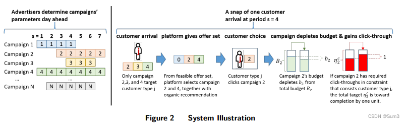
概率单纯形(Probability Simplex)
指的是由一组非负且和为1的随机变量构成的多维空间。在二维空间中,概率单纯形就是一个三角形;在三维空间中,概率单纯形就是一个四面体。具体来说是一个数学空间,上面每个点代表有限个互斥事件之间的概率分布。该空间的每条坐标轴代表一个互斥事件, k − 1 k-1 k−1维单纯形上的每个点在 k k k维空间中的坐标就是其 k k k个互斥事件上的概率分布。每一点的坐标(向量)包含 k k k个元素,各元素非负且和为1。
如下图所示,三个事件发生的概率分布形成一个二维的概率单纯形,上面每个点在三个事件上发生的概率之和为1。
数学形式:给定一个离散集 G G G, G G G上的概率单纯形 △ G \triangle G △G被定义为
△ G = { x ∈ R ∣ G ∣ ∣ x i ⩾ 0 , i = 1 , 2 , … , ∣ G ∣ ; ∑ i = 1 ∣ G ∣ x i = 1 } \triangle G = \big \{ x\in \mathbb{R}^{|G|} |x_i \geqslant0,i=1,2,\dots,|G|;\sum_{i=1}^{|G|}x_i=1 \big \} △G={x∈R∣G∣∣xi⩾0,i=1,2,…,∣G∣;i=1∑∣G∣xi=1}
用 p j s p_j^s pjs表示类型为 j j j的用户在周期 s s s访问平台的概率。那么就可以用 p j s ϕ i j ( S s j ( G s , j ) ) p_j^s\phi_i^j(S_s^j(G_s,j)) pjsϕij(Ssj(Gs,j))表示在周期 s s s访问平台的用户类型为 j j j的用户在广告 i i i上的每个用户的平均点击量。因此, ( 7 ) (7) (7)可等价写成以下的线性规划形式
max G ˉ s 0 s . t . ∑ G s ∈ g s μ s ( G s ) p j s ϕ i j ( S s j ( G s , j ) ) ⩾ α i j ( s ) , ∀ i ∈ N ˉ , j ∈ M ( 8.1 ) ∑ G s ∈ g ~ s μ s ( G s ) = 1 ( 8.2 ) μ s ( G s ) ⩾ 0 , ∀ G ~ s ∈ g ~ s \begin{aligned} & \max_{\bar{G}_s} && 0 \\ & s.t. && \sum_{G_s\in \mathfrak{g}_s}\mu_s(G_s)p_j^s\phi_i^j(S_s^j(G_s,j)) \geqslant \alpha_i^j(s), \forall i\in \bar{\mathcal{N}},j\in\mathcal{M} \quad &(8.1) \\ & && \sum_{G_s\in\tilde{\mathfrak{g}}_s} \mu_s(G_s)=1 & (8.2) \\ & && \mu_s(G_s)\geqslant0,\forall \tilde{G}_s\in \tilde{\mathfrak{g}}_s \end{aligned} Gˉsmaxs.t.0Gs∈gs∑μs(Gs)pjsϕij(Ssj(Gs,j))⩾αij(s),∀i∈Nˉ,j∈MGs∈g~s∑μs(Gs)=1μs(Gs)⩾0,∀G~s∈g~s(8.1)(8.2)
接下来写出其对偶形式
min θ 0 , θ i j { θ 0 − ∑ i ∈ N ˉ , j ∈ M α i j ( s ) θ i j } ( 9.1 ) s . t . ∑ i ∈ N ˉ , j ∈ M p j s ϕ i j ( S s j ( G s , j ) ) θ i j − θ 0 ⩽ 0 , ∀ G ~ s ∈ g ~ s ( 9.2 ) θ i j ⩾ 0 ∀ i ∈ N ˉ , j ∈ M ( 9.3 ) \begin{aligned} & \min_{\theta_0,\theta_i^j} && \big \{ \theta_0-\sum_{i\in\bar{\mathcal{N}},j\in \mathcal{M}}\alpha_i^j(s)\theta_i^j \big \} &(9.1) \\ & s.t. && \sum_{i\in \bar{\mathcal{N}},j\in\mathcal{M}}p_j^s\phi_i^j(S_s^j(G_s,j))\theta_i^j-\theta_0 \leqslant 0, \forall \tilde{G}_s\in \tilde{\mathfrak{g}}_s \quad &(9.2) \\ & &&\theta_i^j\geqslant 0 \forall i\in \bar{\mathcal{N}},j\in\mathcal{M} &(9.3) \end{aligned} θ0,θijmins.t.{θ0−i∈Nˉ,j∈M∑αij(s)θij}i∈Nˉ,j∈M∑pjsϕij(Ssj(Gs,j))θij−θ0⩽0,∀G~s∈g~sθij⩾0∀i∈Nˉ,j∈M(9.1)(9.2)(9.3)
因为主要讨论的是不同的广告推送方案影响的点击量的问题,所以主要讨论的是 θ i j \theta_i^j θij对目标值的影响,然后通过把约束纳入到目标函数的方式将模型 ( 9 ) (9) (9)等价于下面的形式
min θ i j ⩾ 0 { max G s ∈ g s ∑ i ∈ N ˉ , j ∈ M p j s ϕ i j ( S s j ( G s , j ) ) θ i j − ∑ i ∈ N ˉ , j ∈ M α i j ( s ) θ i j } ⩾ 0 ( 10 ) \begin{aligned} & \min_{\theta_i^j \geqslant 0} \left\{ \max_{G_s\in \mathfrak{g}_s} \sum_{i\in \bar{\mathcal{N}},j\in\mathcal{M}} p_j^s\phi_i^j(S_s^j(G_s,j))\theta_i^j - \sum_{i\in\bar{\mathcal{N}},j\in \mathcal{M}}\alpha_i^j(s)\theta_i^j \right\} \geqslant 0 \quad (10) \end{aligned} θij⩾0min⎩ ⎨ ⎧Gs∈gsmaxi∈Nˉ,j∈M∑pjsϕij(Ssj(Gs,j))θij−i∈Nˉ,j∈M∑αij(s)θij⎭ ⎬ ⎫⩾0(10)
然后,从强对偶性可以直接得出,当且仅当 ( 10 ) (10) (10)左侧的最小值大于或等于 0 时, ( 7 ) (7) (7)是可行的。基于这一观察,下面的定理建立了(第二阶段)点进目标 α ( s ) \alpha(s) α(s)的充要条件。
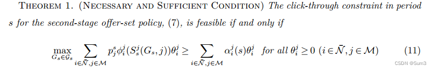
定理1:第二阶段广告推送策略 ( 7 ) (7) (7)在周期 s s s的点击限制是可行的,当且仅当
max G s ∈ g s ∑ i ∈ N ˉ , j ∈ M p j s ϕ i j ( S s j ( G s , j ) ) θ i j ⩾ ∑ i ∈ N ˉ , j ∈ M α i j ( s ) θ i j ( ∀ θ i j ⩾ 0 ) ⩾ 0 ( i ∈ N ˉ , j ∈ M ) ( 11 ) \begin{aligned} & \max_{G_s\in \mathfrak{g}_s} \sum_{i\in \bar{\mathcal{N}},j\in\mathcal{M}} p_j^s\phi_i^j(S_s^j(G_s,j))\theta_i^j \geqslant \sum_{i\in\bar{\mathcal{N}},j\in \mathcal{M}}\alpha_i^j(s)\theta_i^j (\forall \theta_i^j \geqslant 0)\geqslant 0 (i\in\bar{\mathcal{N}},j\in \mathcal{M})\quad (11) \end{aligned} Gs∈gsmaxi∈Nˉ,j∈M∑pjsϕij(Ssj(Gs,j))θij⩾i∈Nˉ,j∈M∑αij(s)θij(∀θij⩾0)⩾0(i∈Nˉ,j∈M)(11)
可以将不等式 ( 11 ) (11) (11)的左侧视为个性化报价集优化问题。具体地说,对于每个客户类型 j j j,寻求提供使来自该客户类型的总收入最大化的广告集合 S s j ∗ S_s^{j^*} Ssj∗,其中广告 i i i的每次点击收入等于 p j s θ i j p^s_j\theta^j_i pjsθij,即
S s j ∗ ( θ ) = arg max s ∈ S j ∑ i ∈ S p j s θ i j ϕ i j ( S ) ( 12 ) \begin{aligned} S_s^{j^*}(\theta)=\arg \max_{s\in \mathcal{S}_j}\sum_{i\in S} p_j^s\theta_i^j\phi_i^j(S) \quad (12) \end{aligned} Ssj∗(θ)=args∈Sjmaxi∈S∑pjsθijϕij(S)(12)
接下来定义 g s ( θ ) : = ∑ j ∈ M max S ∈ S j ∑ i ∈ S p j s θ i j ϕ i j ( S ) g_s(\theta):=\sum_{j\in \mathcal{M}} \max_{S\in S_j} \sum_{i\in S} p_j^s\theta_i^j\phi_i^j(S) gs(θ):=∑j∈MmaxS∈Sj∑i∈Spjsθijϕij(S)表示 ( 11 ) (11) (11)中的左端项,那么可以把点击量期望 ( 8 ) (8) (8)的可行性的等效充分必要条件
min θ i j ⩾ 0 h s ( θ ∣ α ( s ) ) ⩾ 0 ( 13.1 ) w h e r e h s ( θ ∣ α ( s ) ) : = g s ( θ ) − ∑ i ∈ N ˉ , j ∈ M α i j ( s ) θ i j ( 13.2 ) \begin{aligned} & \min_{\theta_i^j \geqslant 0} && h_s(\theta|\alpha(s)) \geqslant 0 &(13.1) \\ & where && h_s(\theta|\alpha(s)):=g_s(\theta) - \sum_{i\in\bar{\mathcal{N}},j\in \mathcal{M}}\alpha_i^j(s)\theta_i^j \quad &(13.2) \end{aligned} θij⩾0minwherehs(θ∣α(s))⩾0hs(θ∣α(s)):=gs(θ)−i∈Nˉ,j∈M∑αij(s)θij(13.1)(13.2)
其中 h s ( ⋅ ∣ α ( s ) ) h_s(\cdot|\alpha(s)) hs(⋅∣α(s))是一个线性函数系列的最大值,对于任何 α ( s ) \alpha(s) α(s)在 θ \theta θ中都是联合凸的。所以在两阶段随机规划模型 ( 4 ) (4) (4)的可行性检验简化为在象限 { θ i j ⩾ 0 : i ∈ N ˉ , ∈ M } \{ \theta_i^j \geqslant 0:i \in \bar{\mathcal{N}}, \in \mathcal{M} \} {θij⩾0:i∈Nˉ,∈M}上最小化一个凸函数 h s ( ⋅ ∣ α ( s ) ) h_s(\cdot|\alpha(s)) hs(⋅∣α(s))。所以当报价集优化问题 ( 12 ) (12) (12)是易于求解的,就可以通过数值检验去检查点击量期望的可行性。
有了第二阶段点击率目标 α ( s ) \alpha(s) α(s)可行性的必要和充分条件 ( 13 ) (13) (13)的描述,就可以把两阶段随机规划 ( 4 ) (4) (4)重新表述为以下凸规划:
max α ∑ s = 1 ∑ ζ s ∑ i ∈ N ˉ r i ∑ j ∈ L i α i j ( s ) ( 14.1 ) s . t . h s ( θ ∣ α ( s ) ) ⩾ 0 ∀ i ∈ N , j ∈ M , s , ( 14.2 ) ∑ s = σ i σ i + K i − 1 ζ s ∑ j ∈ L i α i j ( s ) ⩽ B i T b i , ∀ i ∈ N , ( 14.3 ) ∑ s = σ i σ i + K i − 1 ζ s ∑ j ∈ L i α i j ( s ) ⩾ η i c T , ∀ i ∈ N ˉ , c ⊆ L i ( 14.4 ) \begin{aligned} & \max_{\alpha} && \sum_{s=1}^{\sum}\zeta_s \sum_{i \in \bar {\mathcal{N}}}r_i\sum_{j\in \mathcal{L}_i}\alpha_i^j(s) &(14.1) \\ & s.t. && h_s(\theta|\alpha(s)) \geqslant 0 \forall i\in\mathcal{N},j\in \mathcal{M},s, &(14.2) \\ & &&\sum_{s=\sigma_i}^{\sigma_i+K_i-1}\zeta_s\sum_{j\in\mathcal{L_i}} \alpha_i^j(s) \leqslant \frac{B_i}{Tb_i}, \forall i\in \mathcal{N}, &(14.3) \\ & && \sum_{s=\sigma_i}^{\sigma_i+K_i-1}\zeta_s\sum_{j\in\mathcal{L_i}} \alpha_i^j(s) \geqslant \frac{\eta_i^c}{T}, \forall i\in \bar{\mathcal{N}},c\subseteq \mathcal{L_i} &(14.4) \end{aligned} αmaxs.t.s=1∑∑ζsi∈Nˉ∑rij∈Li∑αij(s)hs(θ∣α(s))⩾0∀i∈N,j∈M,s,s=σi∑σi+Ki−1ζsj∈Li∑αij(s)⩽TbiBi,∀i∈N,s=σi∑σi+Ki−1ζsj∈Li∑αij(s)⩾Tηic,∀i∈Nˉ,c⊆Li(14.1)(14.2)(14.3)(14.4)
( 14 ) (14) (14)在预期意义上表示了最佳点击量目标 α ∗ \alpha^* α∗和相关的松弛后的最佳每用户的点击量。也就是将第一阶段的点击量的期望值与第二阶段的广告推送优化模型联系起来了。但是目前还有两个问题亟需解决:
- 应该如何在每个客户到达时获取报价集以实现最佳点击量目标 α ∗ \alpha^* α∗;
- 带入获取的 α ∗ \alpha^* α∗是否可以获得真正的(非放松的)最优值。
Max-min inequality
对于任何函数 f : Z × W → R f: Z \times W \rightarrow \mathbb{R} f:Z×W→R,都有 sup z ∈ Z inf w ∈ W f ( z , w ) ⩽ inf w ∈ W sup z ∈ Z f ( z , w ) \sup_{z \in Z} \inf_{w \in W}f(z,w) \leqslant \inf_{w \in W} \sup_{z \in Z}f(z,w) supz∈Zinfw∈Wf(z,w)⩽infw∈Wsupz∈Zf(z,w),当等式成立时,可以说 f f f、 W W W和 Z Z Z满足强Max-min inequality属性(或鞍点属性)。例如下图展示的 f ( z , w ) = sin ( z + w ) f(z,w)=\sin (z+w) f(z,w)=sin(z+w)
假设你有一片土地(不必是矩形),考虑横纵两个方向(不必是正交的), z z z或 w w w分别代表了横纵两个方向的坐标,而 f ( z , w ) f(z,w) f(z,w)代表了在该坐标的海拔。假设你把这片土地切成了细横条,在每个横条的最低海拔处放一个红色的鹅卵石作标记(每个横条上可能会有多处标记)。我们在这块土地上随便走,无论这些红石头出现在我们的左方还是右方,抑或恰好在脚下,它们一定有比我们更低或者相同的海拔。
即水平条最低点的最大值不会大于竖直条最高点的最小值。如果我们把这些条带切的更细,我们会看到这个直观的证明在连续条件下成立。我们也会看到这个证明在任何坐标系下都成立。

Minimax theorem
在博弈论的数学领域,极小极大定理是提供保证Max-min inequality也是等式的条件的定理。该定理是在1928年由冯 · 诺依曼(对,就是那个奠定了现代计算机体系结构的冯 · 诺依曼)首次证明并发表的。该理论被认为是博弈论的起点,引用冯·诺依曼的话
“As far as I can see, there could be no theory of games … without that theorem … I thought there was nothing worth publishing until the Minimax Theorem was proved”.
有是紧凸集 X ⊂ R n , Y ⊂ R m X \subset \mathbb{R}^n,Y \subset \mathbb{R}^m X⊂Rn,Y⊂Rm,如果 f : X × Y → R f:X \times Y \rightarrow \mathbb{R} f:X×Y→R是一个连续的凸凹(convex-concave)函数,即:
- f ( ⋅ , y ) : X → R f(\cdot, y):X \rightarrow \mathbb{R} f(⋅,y):X→R对于固定的 y y y是凸的;
- f ( x , ⋅ ) : X → R f(x, \cdot):X \rightarrow \mathbb{R} f(x,⋅):X→R对于固定的 x x x是凹的。
那么有
max x ∈ X max y ∈ Y f ( x , y ) = max y ∈ Y max x ∈ X f ( x , y ) \max_{x\in X} \max_{y \in Y} f(x,y) = \max_{y \in Y} \max_{x\in X} f(x,y) x∈Xmaxy∈Ymaxf(x,y)=y∈Ymaxx∈Xmaxf(x,y)

参考文献
1.Li X, Rong Y, Zhang R P, et al. Online advertisement allocation under customer choices and algorithmic fairness[J]. Available at SSRN 3538755, 2022.
2.全单模矩阵——https://www.zhihu.com/tardis/bd/art/408803563?source_id=1001
3. 概率单纯形——https://www.cnblogs.com/MaplesWCT/p/16299607.html
4.Blackwell Approachability——https://appliedprobability.blog/2017/05/18/blackwells-approachability-theorem/
5.Minimax theorem——https://en.wikipedia.org/wiki/Minimax_theorem
6.Max–min inequality——https://en.wikipedia.org/wiki/Max%E2%80%93min_inequality
7.https://www.zhihu.com/question/51080557/answer/671522746
这篇关于【论文研读】Online Advertisement Allocation in the Presence of Customer Choices-1的文章就介绍到这儿,希望我们推荐的文章对编程师们有所帮助!


![[论文笔记]LLM.int8(): 8-bit Matrix Multiplication for Transformers at Scale](https://img-blog.csdnimg.cn/img_convert/172ed0ed26123345e1773ba0e0505cb3.png)