Python 低通 高通 理想滤波器 巴特沃斯 数字图像处理 频域滤波 图像增强

问题

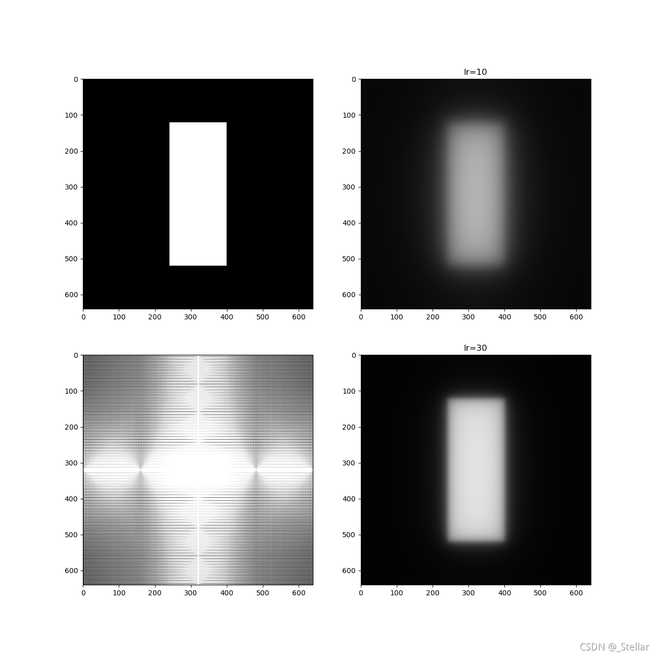
（一）频域低通滤波

1. 产生白条图像 f1(x,y)（640×640 大小，中间亮条宽160，高 400，居中，暗处=0，亮处=255）
2. 设计不同截止频率的理想低通滤波器、Butterworth低通滤波器，对其进行频域增强。观察频域滤波效果，并解释之。

（二）频域高通滤波

1. 设计不同截止频率的理想高通滤波器、Butterworth高通滤波器，对上述白条图像进行频域增强。观察频域滤波效果，并解释之。
2. 设计不同截止频率的理想高通滤波器、Butterworth高通滤波器，对含高斯噪声的lena图像进行频域增强。观察频域滤波效果，并解释之。

代码

import numpy as np
from PIL import Image
import matplotlib.pyplot as plt"""
（一）频域低通滤波
产生如图所示图象 f1(x,y)（64×64 大小，中间亮条宽16，高 40，居中，暗处=0，亮处=255）
产生实验四中的白条图像。
设计不同截止频率的理想低通滤波器、Butterworth低通滤波器，对其进行频域增强。
观察频域滤波效果，并解释之。
"""def pro_11():def ideal_low_filter(lr, cr, cc, img):tmp = np.zeros((img.shape[0], img.shape[1]))for i in range(img.shape[0]):for j in range(img.shape[1]):tmp[i, j] = (1 if np.sqrt((i - cr) ** 2 + (j - cc) ** 2) <= lr else 0)return tmp# 产生白条图像im_arr = np.zeros((640, 640))for i in range(im_arr.shape[0]):for j in range(im_arr.shape[1]):if 120 < i < 520 and 240 < j < 400:im_arr[i, j] = 255im_ft2 = np.fft.fft2(np.array(im_arr))  # 白条图二维傅里叶变换矩阵im_ft2_shift = np.fft.fftshift(im_ft2)r, c = im_arr.shape[0], im_arr.shape[1]cr, cc = r // 2, c // 2  # 频谱中心# 理想滤波器ideal_filter1 = ideal_low_filter(10, cr, cc, im_ft2_shift)ideal_filter2 = ideal_low_filter(30, cr, cc, im_ft2_shift)# 求经理想低通滤波器后的图像tmp = im_ft2_shift * ideal_filter1irreversed_im_ft2 = np.fft.ifft2(tmp)tmp2 = im_ft2_shift * ideal_filter2irreversed_im_ft22 = np.fft.ifft2(tmp2)plt.figure(figsize=(13, 13))plt.subplot(221)plt.imshow(Image.fromarray(np.abs(im_arr)))plt.subplot(223)plt.imshow(Image.fromarray(np.abs(im_ft2_shift)))plt.subplot(222)plt.title("lr=10")plt.imshow(Image.fromarray(np.abs(irreversed_im_ft2)))plt.subplot(224)plt.title("lr=30")plt.imshow(Image.fromarray(np.abs(irreversed_im_ft22)))plt.show()def pro_12():def butterworth(lr, cr, cc, n, img):tmp = np.zeros((img.shape[0], img.shape[1]))for i in range(img.shape[0]):for j in range(img.shape[1]):tmp[i, j] = 1 / (1 + np.sqrt((i - cr) ** 2 + (j - cc) ** 2) / lr) ** (2 * n)return tmp# 产生白条图像im_arr = np.zeros((640, 640))for i in range(im_arr.shape[0]):for j in range(im_arr.shape[1]):if 120 < i < 520 and 240 < j < 400:im_arr[i, j] = 255im_ft2 = np.fft.fft2(np.array(im_arr))  # 白条图二维傅里叶变换矩阵im_ft2_shift = np.fft.fftshift(im_ft2)r, c = im_arr.shape[0], im_arr.shape[1]cr, cc = r // 2, c // 2  # 频谱中心# 理想滤波器butterworth1 = butterworth(10, cr, cc, 2, im_arr)butterworth2 = butterworth(30, cr, cc, 2, im_arr)# 求经理想低通滤波器后的图像tmp = im_ft2_shift * butterworth1irreversed_im_ft2 = np.fft.ifft2(tmp)tmp2 = im_ft2_shift * butterworth2irreversed_im_ft22 = np.fft.ifft2(tmp2)plt.figure(figsize=(13, 13))plt.subplot(221)plt.imshow(Image.fromarray(np.abs(im_arr)))plt.subplot(223)plt.imshow(Image.fromarray(np.abs(im_ft2_shift)))plt.subplot(222)plt.title("lr=10")plt.imshow(Image.fromarray(np.abs(irreversed_im_ft2)))plt.subplot(224)plt.title("lr=30")plt.imshow(Image.fromarray(np.abs(irreversed_im_ft22)))plt.show()def pro_12():def ideal_low_filter(lr, cr, cc, img):tmp = np.zeros((img.shape[0], img.shape[1]))for i in range(img.shape[0]):for j in range(img.shape[1]):tmp[i, j] = (1 if np.sqrt((i - cr) ** 2 + (j - cc) ** 2) <= lr else 0)return tmpdef butterworth(lr, cr, cc, n, img):tmp = np.zeros((img.shape[0], img.shape[1]))for i in range(img.shape[0]):for j in range(img.shape[1]):tmp[i, j] = 1 / (1 + np.sqrt((i - cr) ** 2 + (j - cc) ** 2) / lr) ** (2 * n)return tmpdef gauss_noise(img, sigma):temp_img = np.float64(np.copy(img))h = temp_img.shape[0]w = temp_img.shape[1]noise = np.random.randn(h, w) * sigmanoisy_img = np.zeros(temp_img.shape, np.float64)if len(temp_img.shape) == 2:noisy_img = temp_img + noiseelse:noisy_img[:, :, 0] = temp_img[:, :, 0] + noisenoisy_img[:, :, 1] = temp_img[:, :, 1] + noisenoisy_img[:, :, 2] = temp_img[:, :, 2] + noise# noisy_img = noisy_img.astype(np.uint8)return noisy_imglena = np.array(Image.open("lena_gray_512.tif"))noise_lena = gauss_noise(lena, 25)noise_lena_fft2 = np.fft.fft2(noise_lena)noise_lena_fft2_shift = np.fft.fftshift(noise_lena_fft2)r, c = lena.shape[0], lena.shape[1]cr, cc = r // 2, c // 2  # 频谱中心butterworth1 = butterworth(30, cr, cc, 2, lena)butterworth2 = butterworth(50, cr, cc, 2, lena)ideal_filter1 = ideal_low_filter(10, cr, cc, noise_lena_fft2_shift)ideal_filter2 = ideal_low_filter(30, cr, cc, noise_lena_fft2_shift)btmp1 = noise_lena_fft2_shift * butterworth1blena_ift21 = np.fft.ifft2(btmp1)btmp2 = noise_lena_fft2_shift * butterworth2blena_ift22 = np.fft.ifft2(btmp2)itmp1 = noise_lena_fft2_shift * ideal_filter1ilena_ift21 = np.fft.ifft2(itmp1)itmp2 = noise_lena_fft2_shift * ideal_filter2ilena_ift22 = np.fft.ifft2(itmp2)plt.figure(figsize=(13, 13))plt.subplot(221)plt.title("Butterworth Filter: lr=30/100")plt.imshow(Image.fromarray(np.abs(blena_ift21)))plt.subplot(223)plt.imshow(Image.fromarray(np.abs(blena_ift22)))plt.subplot(222)plt.title("Ideal Filter: lr=10/30")plt.imshow(Image.fromarray(np.abs(ilena_ift21)))plt.subplot(224)plt.imshow(Image.fromarray(np.abs(ilena_ift22)))plt.show()"""
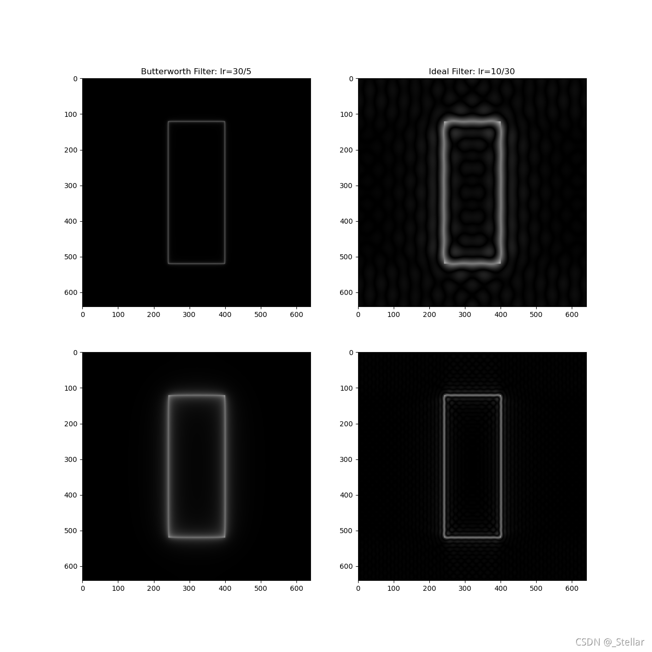
（二）频域高通滤波
1. 设计不同截止频率的理想高通滤波器、Butterworth高通滤波器，对上述白条图像进行频域增强。观察频域滤波效果，并解释之。
2. 设计不同截止频率的理想高通滤波器、Butterworth高通滤波器，对含高斯噪声的lena图像进行频域增强。观察频域滤波效果，并解释之。
"""def pro_2():def ideal_high_filter(lr, cr, cc, img):tmp = np.zeros((img.shape[0], img.shape[1]))for i in range(img.shape[0]):for j in range(img.shape[1]):tmp[i, j] = (0 if np.sqrt((i - cr) ** 2 + (j - cc) ** 2) <= lr else 1)return tmpdef butterworth_high(lr, cr, cc, n, img):tmp = np.zeros((img.shape[0], img.shape[1]))for i in range(img.shape[0]):for j in range(img.shape[1]):tmp[i, j] = 1 / (1 + lr / np.sqrt((i - cr) ** 2 + (j - cc) ** 2)) ** (2 * n)return tmpdef gauss_noise(img, sigma):temp_img = np.float64(np.copy(img))h = temp_img.shape[0]w = temp_img.shape[1]noise = np.random.randn(h, w) * sigmanoisy_img = np.zeros(temp_img.shape, np.float64)if len(temp_img.shape) == 2:noisy_img = temp_img + noiseelse:noisy_img[:, :, 0] = temp_img[:, :, 0] + noisenoisy_img[:, :, 1] = temp_img[:, :, 1] + noisenoisy_img[:, :, 2] = temp_img[:, :, 2] + noise# noisy_img = noisy_img.astype(np.uint8)return noisy_imgdef lena_proceed():lena = np.array(Image.open("lena_gray_512.tif"))noise_lena = gauss_noise(lena, 25)noise_lena_fft2 = np.fft.fft2(noise_lena)noise_lena_fft2_shift = np.fft.fftshift(noise_lena_fft2)r, c = lena.shape[0], lena.shape[1]cr, cc = r // 2, c // 2  # 频谱中心butterworth1 = butterworth_high(10, cr, cc, 1, lena)butterworth2 = butterworth_high(5, cr, cc, 1, lena)ideal_filter1 = ideal_high_filter(10, cr, cc, noise_lena_fft2_shift)ideal_filter2 = ideal_high_filter(30, cr, cc, noise_lena_fft2_shift)btmp1 = noise_lena_fft2_shift * butterworth1blena_ift21 = np.fft.ifft2(btmp1)btmp2 = noise_lena_fft2_shift * butterworth2blena_ift22 = np.fft.ifft2(btmp2)itmp1 = noise_lena_fft2_shift * ideal_filter1ilena_ift21 = np.fft.ifft2(itmp1)itmp2 = noise_lena_fft2_shift * ideal_filter2ilena_ift22 = np.fft.ifft2(itmp2)plt.figure(figsize=(13, 13))plt.subplot(221)plt.title("Butterworth Filter: lr=30/5")plt.imshow(Image.fromarray(np.abs(blena_ift21)))plt.subplot(223)plt.imshow(Image.fromarray(np.abs(blena_ift22)))plt.subplot(222)plt.title("Ideal Filter: lr=10/30")plt.imshow(Image.fromarray(np.abs(ilena_ift21)))plt.subplot(224)plt.imshow(Image.fromarray(np.abs(ilena_ift22)))plt.show()def white_bar_proceed():# 产生白条图像im_arr = np.zeros((640, 640))for i in range(im_arr.shape[0]):for j in range(im_arr.shape[1]):if 120 < i < 520 and 240 < j < 400:im_arr[i, j] = 255im_ft2 = np.fft.fft2(np.array(im_arr))  # 白条图二维傅里叶变换矩阵im_ft2_shift = np.fft.fftshift(im_ft2)r, c = im_arr.shape[0], im_arr.shape[1]cr, cc = r // 2, c // 2  # 频谱中心butterworth1 = butterworth_high(30, cr, cc, 1, im_arr)butterworth2 = butterworth_high(5, cr, cc, 1, im_arr)ideal_filter1 = ideal_high_filter(10, cr, cc, im_ft2_shift)ideal_filter2 = ideal_high_filter(30, cr, cc, im_ft2_shift)btmp1 = im_ft2_shift * butterworth1blena_ift21 = np.fft.ifft2(btmp1)btmp2 = im_ft2_shift * butterworth2blena_ift22 = np.fft.ifft2(btmp2)itmp1 = im_ft2_shift * ideal_filter1ilena_ift21 = np.fft.ifft2(itmp1)itmp2 = im_ft2_shift * ideal_filter2ilena_ift22 = np.fft.ifft2(itmp2)plt.figure(figsize=(13, 13))plt.subplot(221)plt.title("Butterworth Filter: lr=30/5")plt.imshow(Image.fromarray(np.abs(blena_ift21)))plt.subplot(223)plt.imshow(Image.fromarray(np.abs(blena_ift22)))plt.subplot(222)plt.title("Ideal Filter: lr=10/30")plt.imshow(Image.fromarray(np.abs(ilena_ift21)))plt.subplot(224)plt.imshow(Image.fromarray(np.abs(ilena_ift22)))plt.show()lena_proceed()white_bar_proceed()if __name__ == '__main__':pro_11()pro_12()pro_2()

结果