一张图看明白Self-Attention机制

镇楼图

Illustrated: Self-Attention

A step-by-step guide to self-attention with illustrations and code

---

这篇文章非常通俗易懂，虽然是英语，很容易就能够看懂，我就不给大家翻译了。我看了很多self-attention的内容，目前来说这篇文章写的非常清晰，所以我搬到了CSDN上，能够帮助更多人理解Self_Attention。

原文外网博文地址：Illustrated: Self-Attention

---

Transformer-based architectures, which are primarily used in modelling language understanding tasks, eschew recurrence in neural networks and instead trust entirely on self-attention mechanisms to draw global dependencies between inputs and outputs

1. Illustrations

The illustrations are divided into the following steps:

1. Prepare inputs
2. Initialise weights
3. Derive key, query and value
4. Calculate attention scores for Input 1
5. Calculate softmax
6. Multiply scores with values
7. Sum weighted values to get Output 1
8. Repeat steps 4–7 for Input 2 & Input 3

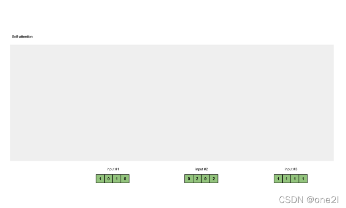
Step 1: Prepare inputs

We start with 3 inputs for this tutorial, each with dimension 4.

Input 1: [1, 0, 1, 0] 
Input 2: [0, 2, 0, 2]
Input 3: [1, 1, 1, 1]

Step 2: Initialise weights

Every input must have three representations (see diagram below). These representations are called key (orange), query (red), and value (purple). For this example, let’s take that we want these representations to have a dimension of 3. Because every input has a dimension of 4, each set of the weights must have a shape of 4×3.

Note
We’ll see later that the dimension of value *is also the output dimension.

To obtain these representations, every input (green) is multiplied with a set of weights for keys, a set of weights for querys (I know that’s not the correct spelling), and a set of weights for values. In our example, we initialise the three sets of weights as follows.

Weights for key:

[[0, 0, 1],[1, 1, 0],[0, 1, 0],[1, 1, 0]]

Weights for query:

[[1, 0, 1],[1, 0, 0],[0, 0, 1],[0, 1, 1]]

Weights for value:

[[0, 2, 0],[0, 3, 0],[1, 0, 3],[1, 1, 0]]

Notes
In a neural network setting, these weights are usually small numbers, initialised randomly using an appropriate random distribution like Gaussian, Xavier and Kaiming distributions. This initialisation is done once before training.

Step 3: Derive key, query and value

Now that we have the three sets of weights, let’s obtain the key, query and value representations for every input

Key representation for Input 1:

               [0, 0, 1]
[1, 0, 1, 0] x [1, 1, 0] = [0, 1, 1][0, 1, 0][1, 1, 0]

Use the same set of weights to get the key representation for Input 2:

               [0, 0, 1]
[0, 2, 0, 2] x [1, 1, 0] = [4, 4, 0][0, 1, 0][1, 1, 0]

Use the same set of weights to get the key representation for Input 3:

               [0, 0, 1]
[1, 1, 1, 1] x [1, 1, 0] = [2, 3, 1][0, 1, 0][1, 1, 0]

A faster way is to vectorise the above operations:

               [0, 0, 1]
[1, 0, 1, 0]   [1, 1, 0]   [0, 1, 1]
[0, 2, 0, 2] x [0, 1, 0] = [4, 4, 0]
[1, 1, 1, 1]   [1, 1, 0]   [2, 3, 1]

Let’s do the same to obtain the value representations for every input:

               [0, 2, 0]
[1, 0, 1, 0]   [0, 3, 0]   [1, 2, 3] 
[0, 2, 0, 2] x [1, 0, 3] = [2, 8, 0]
[1, 1, 1, 1]   [1, 1, 0]   [2, 6, 3]

and finally the query representations:

               [1, 0, 1]
[1, 0, 1, 0]   [1, 0, 0]   [1, 0, 2]
[0, 2, 0, 2] x [0, 0, 1] = [2, 2, 2]
[1, 1, 1, 1]   [0, 1, 1]   [2, 1, 3]

Notes
In practice, a bias vector may be added to the product of matrix multiplication.

Step 4: Calculate attention scores for Input 1

To obtain attention scores, we start with taking a dot product between Input 1’s query (red) with all keys (orange), including itself. Since there are 3 key representations (because we have 3 inputs), we obtain 3 attention scores (blue).

            [0, 4, 2]
[1, 0, 2] x [1, 4, 3] = [2, 4, 4][1, 0, 1]

Notice that we only use the query from Input 1. Later we’ll work on repeating this same step for the other querys.

Note
The above operation is known as dot product attention, one of the several score functions. Other score functions include scaled dot product and additive/concat.

Step 5: Calculate softmax
Take the softmax across these attention scores (blue).

softmax([2, 4, 4]) = [0.0, 0.5, 0.5]

Note that we round off to 1 decimal place here for readability.

Step 6: Multiply scores with values

The softmaxed attention scores for each input (blue) is multiplied by its corresponding value (purple). This results in 3 alignment vectors (yellow). In this tutorial, we’ll refer to them as weighted values.

1: 0.0 * [1, 2, 3] = [0.0, 0.0, 0.0]
2: 0.5 * [2, 8, 0] = [1.0, 4.0, 0.0]
3: 0.5 * [2, 6, 3] = [1.0, 3.0, 1.5]

Step 7: Sum weighted values to get Output 1

Take all the weighted values (yellow) and sum them element-wise:

  [0.0, 0.0, 0.0]
+ [1.0, 4.0, 0.0]
+ [1.0, 3.0, 1.5]
-----------------
= [2.0, 7.0, 1.5]

Step 8: Repeat for Input 2 & Input 3

Now that we’re done with Output 1, we repeat Steps 4 to 7 for Output 2 and Output 3. I trust that I can leave you to work out the operations yourself 👍🏼

2. Code

Here is the code in PyTorch 🤗, a popular deep learning framework in Python. To enjoy the APIs for @ operator, .T and None indexing in the following code snippets, make sure you’re on Python≥3.6 and PyTorch 1.3.1. Just follow along and copy-paste these in a Python/IPython REPL or Jupyter Notebook.

Step 1: Prepare inputs

import torchx = [[1, 0, 1, 0], # Input 1[0, 2, 0, 2], # Input 2[1, 1, 1, 1]  # Input 3]
x = torch.tensor(x, dtype=torch.float32)

Step 2: Initialise weights

w_key = [[0, 0, 1],[1, 1, 0],[0, 1, 0],[1, 1, 0]
]
w_query = [[1, 0, 1],[1, 0, 0],[0, 0, 1],[0, 1, 1]
]
w_value = [[0, 2, 0],[0, 3, 0],[1, 0, 3],[1, 1, 0]
]
w_key = torch.tensor(w_key, dtype=torch.float32)
w_query = torch.tensor(w_query, dtype=torch.float32)
w_value = torch.tensor(w_value, dtype=torch.float32)

Step 3: Derive key, query and value

keys = x @ w_key
querys = x @ w_query
values = x @ w_valueprint(keys)
# tensor([[0., 1., 1.],
#         [4., 4., 0.],
#         [2., 3., 1.]])print(querys)
# tensor([[1., 0., 2.],
#         [2., 2., 2.],
#         [2., 1., 3.]])print(values)
# tensor([[1., 2., 3.],
#         [2., 8., 0.],
#         [2., 6., 3.]])

Step 4: Calculate attention scores

attn_scores = querys @ keys.T# tensor([[ 2.,  4.,  4.],  # attention scores from Query 1
#         [ 4., 16., 12.],  # attention scores from Query 2
#         [ 4., 12., 10.]]) # attention scores from Query 3

Step 5: Calculate softmax

from torch.nn.functional import softmaxattn_scores_softmax = softmax(attn_scores, dim=-1)
# tensor([[6.3379e-02, 4.6831e-01, 4.6831e-01],
#         [6.0337e-06, 9.8201e-01, 1.7986e-02],
#         [2.9539e-04, 8.8054e-01, 1.1917e-01]])# For readability, approximate the above as follows
attn_scores_softmax = [[0.0, 0.5, 0.5],[0.0, 1.0, 0.0],[0.0, 0.9, 0.1]
]
attn_scores_softmax = torch.tensor(attn_scores_softmax)

Step 6: Multiply scores with values

weighted_values = values[:,None] * attn_scores_softmax.T[:,:,None]# tensor([[[0.0000, 0.0000, 0.0000],
#          [0.0000, 0.0000, 0.0000],
#          [0.0000, 0.0000, 0.0000]],
# 
#         [[1.0000, 4.0000, 0.0000],
#          [2.0000, 8.0000, 0.0000],
#          [1.8000, 7.2000, 0.0000]],
# 
#         [[1.0000, 3.0000, 1.5000],
#          [0.0000, 0.0000, 0.0000],
#          [0.2000, 0.6000, 0.3000]]])

Step 7: Sum weighted values

outputs = weighted_values.sum(dim=0)# tensor([[2.0000, 7.0000, 1.5000],  # Output 1
#         [2.0000, 8.0000, 0.0000],  # Output 2
#         [2.0000, 7.8000, 0.3000]]) # Output 3

Note
PyTorch has provided an API for this callenn.MultiheadAttention. However, this API requires that you feed in key, query and value PyTorch tensors. Moreover, the outputs of this module undergo a linear transformation.