perl 传单引号_使用geopandas和传单在python和r中绘制精美的地理图

There are several geographic libraries that are available for plotting location information on a map. I’ve previously written about the same topic here but since then I’ve used these libraries more extensively as well as got introduced to new ones. After using and examining several libraries, I found that GeoPandas and the Leaflet libraries are two of the most easy to use and highly customizable libraries. The code is available as a GitHub repo:

有几个地理库可用于在地图上绘制位置信息。 我以前在这里曾写过同一主题，但是从那时起，我就更广泛地使用了这些库，并且将它们引入了新库。 使用并检查了几个库之后，我发现GeoPandas和Leaflet库是最易于使用和高度可定制的两个库。 该代码可作为GitHub存储库提供：

数据集 (Dataset)

The dataset is taken from Kaggle. It includes the population density (population per square Km) for various countries across the world. The dataset includes the values ranging from 1961 to 2015.

该数据集取自Kaggle 。 它包括世界各国的人口密度(每平方千米人口)。 数据集包括从1961年到2015年的值。

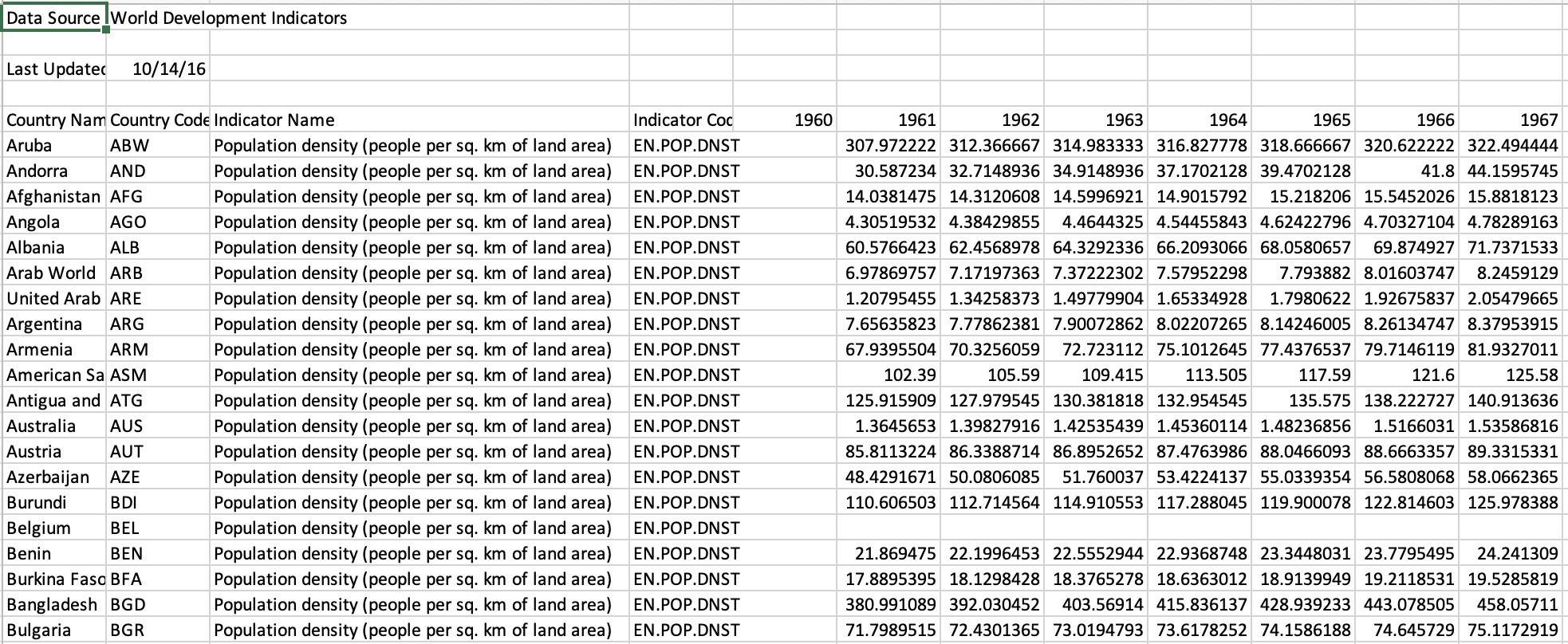
The figure above shows that we need to skip the first 4 rows when reading in the dataset, so we directly start with the data. Columns such as “1960” are empty and hence they can be removed. Also, data for some countries like Belgium is missing so we’ll remove these records from our collection.

上图显示，在读取数据集时，我们需要跳过前4行，因此我们直接从数据开始。 诸如“ 1960”的列为空，因此可以将其删除。 另外，某些国家(例如比利时)的数据丢失了，因此我们将从集合中删除这些记录。

使用GeoPandas的静态图(在Python中) (Static plots using GeoPandas (in Python))

导入库 (Import libraries)

We’ll import the library pandas to read the dataset and then plot the maps using geopandas. Note that to remove unnecessary warnings, I added the specific command.

我们将导入库pandas以读取数据集，然后使用geopandas绘制地图。 请注意，为消除不必要的警告，我添加了特定命令。

import pandas as pd
import geopandas as gpdimport warnings
warnings.filterwarnings('ignore')%matplotlib inline

导入数据集(Import dataset)

Next, we’ll import the dataset. As mentioned before, I skip the first 4 rows.

接下来，我们将导入数据集。 如前所述，我跳过了前4行。

dataset = pd.read_csv("data/dataset.csv", skiprows=4)
dataset = dataset.drop(["Indicator Name", "Indicator Code", "1960", "2016", "Unnamed: 61"], axis = 1)
dataset = dataset.dropna(how = 'any')
dataset["avgPopulationDensity"] = dataset.iloc[:, 2:].mean(axis = 1)
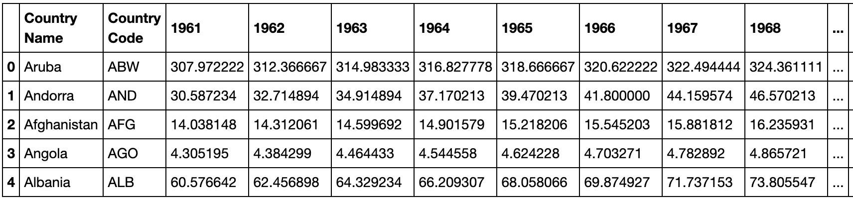
dataset.head()

I remove all the extra columns that I don’t need (“Indicator Name”, “Indicator Code”, “1960”, “2016”, “Unnamed: 61”) using the drop() method. I remove all records with any NULL values using dropna()and finally calculate the average population density across years 1961 to 2015 into a new column avgPopulationDensity.

我使用drop()方法删除了所有不需要的额外列(“指标名称”，“指标代码”，“ 1960”，“ 2016”，“未命名：61”)。 我使用dropna()删除所有具有任何NULL值的记录，最后将1961年至2015年之间的平均人口密度计算到新列avgPopulationDensity 。

绘图数据(Plot data)

We first load in the world baseplot directly from geopandas and then merge the dataset we refined above with this baseplot data. Then, we simply plot th data world shaded by the values in the avgPopulationDensity column. We shade the countries in the Reds colormap which means countries with higher average population densities are darker than other countries.

我们首先直接从geopandas加载世界基准图，然后将我们在上面精炼的数据集与此基准图数据合并。 然后，我们简单地绘制由avgPopulationDensity列中的值阴影的数据world 。 我们在“ Reds配色图中为国家/地区加阴影，这意味着平均人口密度较高的国家/地区比其他国家更暗。

world = gpd.read_file(gpd.datasets.get_path('naturalearth_lowres'))
world = world.merge(dataset, how = 'left', left_on = 'iso_a3', right_on = 'Country Code')
world.plot(column = 'avgPopulationDensity', edgecolor = 'black',figsize = (16, 16),cmap = 'Reds')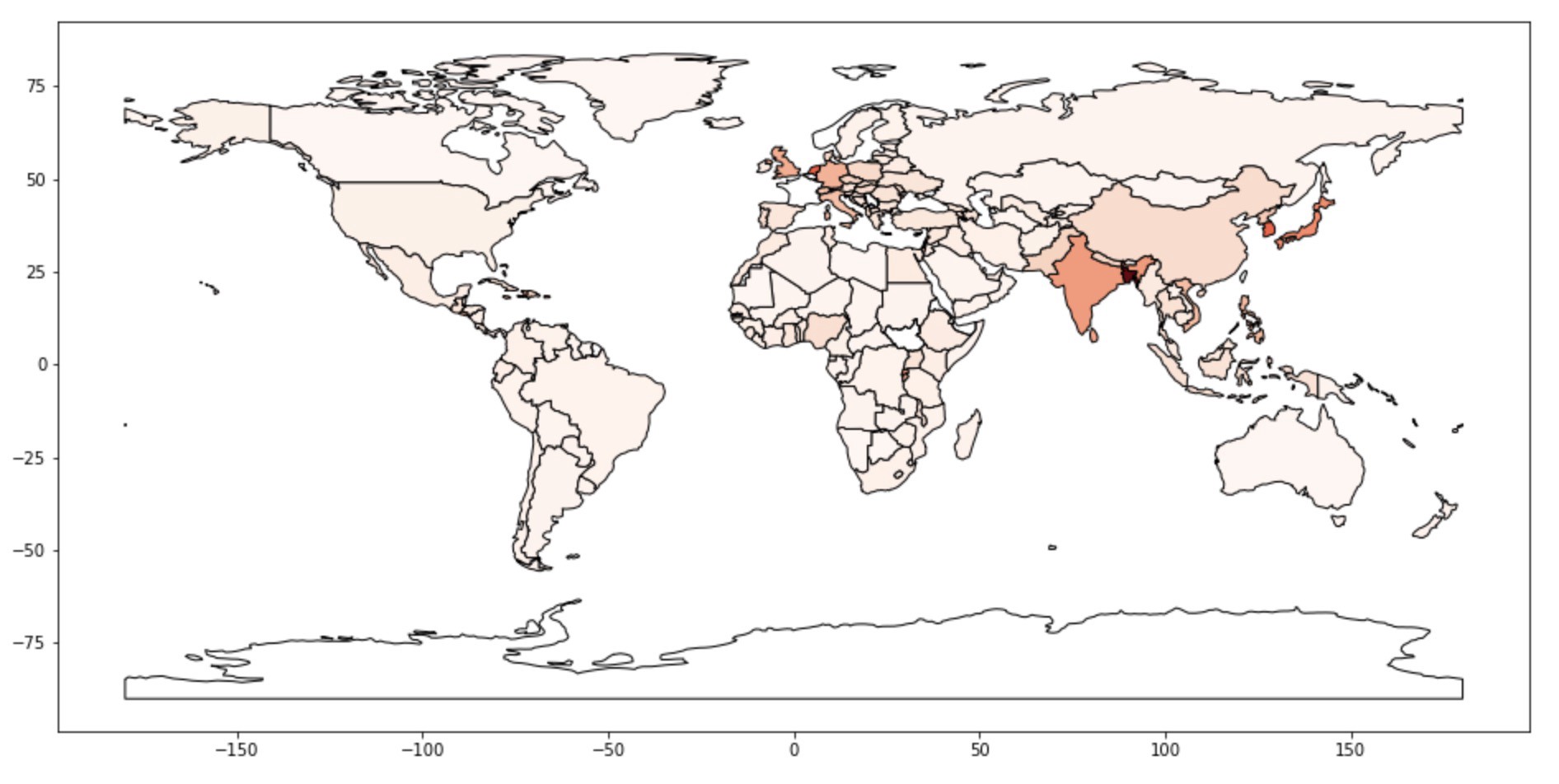

We can clearly see that countries in Asia have more population density values especially India, Bangladesh, Korea and Japan.

我们可以清楚地看到，亚洲国家的人口密度值更高，尤其是印度，孟加拉国，韩国和日本。

使用Leaflet的交互式图(在R中) (Interactive plots using Leaflet (in R))

导入库 (Import libraries)

We’ll load in the leaflet library for generating plots and the sf library for reading in shapefiles.

我们将加载用于生成图形的leaflet库，并加载用于读取shapefile的sf库。

library(leaflet)
library(sf)

导入数据集(Import dataset)

Just like in Python, we’d import in the dataset skipping first 4 rows, remove extra columns, remove rows with missing values and create the avgPopulationDensity column.

就像在Python中一样，我们将跳过前4行导入数据集中，删除多余的列，删除缺少值的行并创建avgPopulationDensity列。

dataset <- read.csv("data/dataset.csv", skip = 4)
dataset[, c("Indicator.Name", "Indicator.Code", "X1960", "X2016", "X")] <- NULL
dataset <- dataset[complete.cases(dataset), ]
dataset["avgPopulationDensity"] <- rowSums(dataset[,3:57])

It’s important that we also load in the shapefile needed for the plotting. Thus, we use the st_read method and merge the dataset with this shapefile into a variable named shapes.

重要的是，我们还要加载绘图所需的shapefile。 因此，我们使用st_read方法并将具有此shapefile的数据集合并到一个名为shapes的变量中。

shapes <- st_read("data/countries_shp/countries.shp")
shapes <- merge(shapes, dataset, by.x = 'ISO3', by.y = 'Country.Code')

绘图数据(Plot data)

Before we plot the data, we first define the color palette we want to use. I defined the shades of red for various bins and based on that I will shade the resultant plot. As this is a custom palette, it’s colors will be different from the one we see in the GeoPandas plot.

在绘制数据之前，我们首先定义要使用的调色板。 我为各种垃圾箱定义了红色阴影，并以此为基础绘制了结果图。 由于这是一个自定义调色板，因此其颜色将与我们在GeoPandas图中看到的颜色不同。

colors <- c("#8B0000","#FF0000", "#FFA07A")
bins <- c(100000, 20000, 5000, 0)color_pal <- leaflet::colorBin(colors, domain = shapes$avgPopulationDensity, bins = bins)

Next, we plot the leaflet geoplot. The leaflet() starts creating the plot and addTiles() adds the tiles for the countries. Next, we set the view of the map by defining the latitude and longitude values as well as the zoom so we can see the whole map at once. We can change the values if needed but as it is an interactive map, we can do so dynamically too.

接下来，我们绘制传单地理图。 leaflet()开始创建图， addTiles()添加国家/地区的图块。 接下来，我们通过定义纬度和经度值以及缩放比例来设置地图视图，以便我们可以一次查看整个地图。 我们可以根据需要更改值，但由于它是一个交互式地图，因此也可以动态更改。

leaflet(shapes) %>% addTiles() %>%setView(lat = 10, lng = 0, zoom = 1) %>%addPolygons(fillColor = ~color_pal(shapes$avgPopulationDensity),fillOpacity = 0.7,label = shapes$Country.Name,stroke = TRUE,color = 'black',weight = 1,opacity = 1)

Finally, based on the avgPopulationDensity column, we color grade the whole plot and attach country names as labels. We customize the look of each country by adding in strokes (STROKE = TRUE), and then setting them to be black with weight = 1, defining the width of each boundary.

最后，基于avgPopulationDensity列，我们对整个绘图进行颜色分级，并附加国家名称作为标签。 我们通过添加笔画( STROKE = TRUE )，然后将它们设置为weight = 1 black ，定义每个边界的宽度，来自定义每个国家/地区的外观。

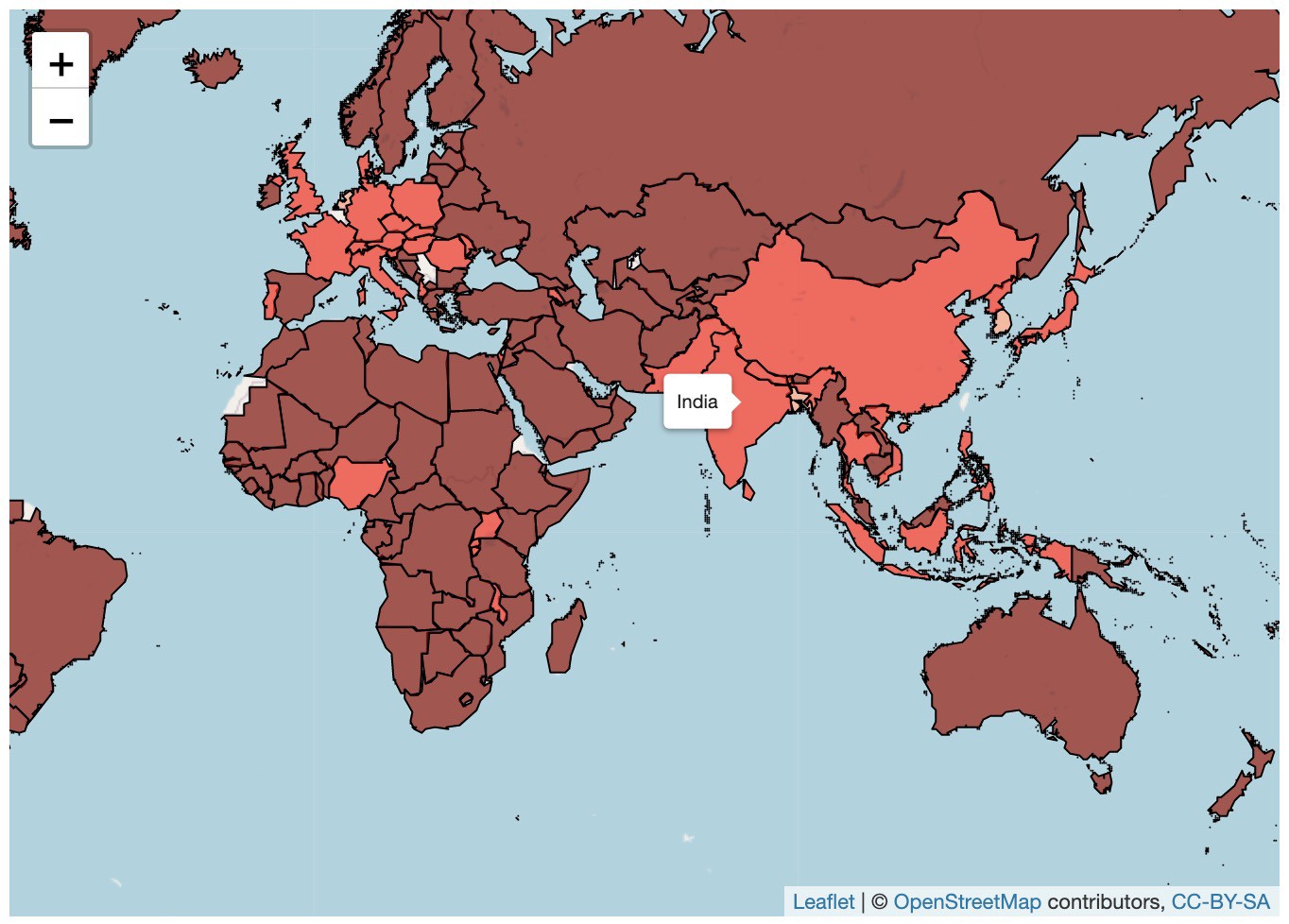
We observe that countries in Asia like India, Bangladesh, China, Japan and others have high population densities than other countries.

我们观察到，印度，孟加拉国，中国，日本等亚洲国家的人口密度比其他国家高。

结论 (Conclusion)

From the two examples above, we see how easy it is to create beautiful static and dynamic geographic plots. Plus, there are tons of customizations that we can add.

从上面的两个示例中，我们看到了创建漂亮的静态和动态地理图非常容易。 另外，我们可以添加大量自定义设置。

If you have any suggestions, questions or ideas, please let me know down below.

如果您有任何建议，问题或想法，请在下面告诉我。