本文主要是介绍头颈肿瘤在PET/CT中的分割:HECKTOR挑战赛| 文献速递-深度学习肿瘤自动分割,希望对大家解决编程问题提供一定的参考价值,需要的开发者们随着小编来一起学习吧!
Title
题目
Head and neck tumor segmentation in PET/CT: The HECKTOR challenge
头颈肿瘤在PET/CT中的分割:HECKTOR挑战赛
01
文献速递介绍
高通量医学影像分析,常被称为放射组学,已显示出其在揭示定量影像生物标志物与癌症预后之间关系的潜力,包括在头颈(H&N)癌症的背景下(Vallieres等,2017;Bogowicz等,2017)。头颈癌是发病率第五高的癌症(Parkin等,2005),其治疗通常基于放射治疗与系统治疗(例如赛妥昔单抗)的组合(Bonner等,2010)。然而,治疗这种癌症仍具挑战性,因为大约40%的患者在治疗后的前两年内会发生局部失败(Chajon等,2013)。开发非侵入性和个性化的方法(例如放射组学)对于改善疾病特征化至关重要,并有望导致基于表型肿瘤特征的更有针对性的治疗。2-[18F]氟代脱氧葡萄糖正电子发射断层扫描(FDG-PET)和计算机断层扫描(CT)在疾病特征化中占有特殊地位,因为它们包含有关癌症的代谢和解剖的互补信息。此外,它们用于头颈癌的初步分期和随访。因此,这些模式易于用于基于临床获得的图像创建和评估放射组学模型。典型的放射组学分析依赖于在已勾画的病变或兴趣体积(VOI)内的局部特征提取(Lambin等,2017;Gillies等,2016)。
阻碍强大模型开发的原因之一是耗时且容易出错的手动勾画这些VOI。为此,自动分割头颈原发肿瘤(GTVt)和淋巴结(GTVn)的总肿瘤体积构成了一种非常有前景的方法,用于标注和分析非常大的队列,这对于实现放射组学模型的强大和可重复性验证至关重要。此外,自动分割还有潜力让放射肿瘤科医生通过减少肿瘤勾画所需时间以及改善观察者间的再现性,来提高治疗计划的效率。
头颈肿瘤(HECKTOR)挑战赛的目标是建立并评估最佳性能方法,用于头颈病变分割,同时利用联合PET/CT的丰富的双模态信息。在这一挑战赛的首届中,参与者被要求开发用于分割患有口咽癌患者FDG-PET/CT图像上的GTVt2的自动方法。值得注意的是,要成为正式排名的一部分,参与者必须提供一篇描述其方法的论文。
Abstract
摘要
This paper relates the post-analysis of the first edition of the HEad and neCK TumOR (HECKTOR) challenge. This challenge was held as a satellite event of the 23rd International Conference on Medical ImageComputing and Computer-Assisted Intervention (MICCAI) 2020, and was the first of its kind focusing onlesion segmentation in combined FDG-PET and CT image modalities. The challenge’s task is the automatic segmentation of the Gross Tumor Volume (GTV) of Head and Neck (H&N) oropharyngeal primarytumors in FDG-PET/CT images. To this end, the participants were given a training set of 201 cases fromfour different centers and their methods were tested on a held-out set of 53 cases from a fifth center.The methods were ranked according to the Dice Score Coefficient (DSC) averaged across all test cases. Anadditional inter-observer agreement study was organized to assess the difficulty of the task from a human perspective. 64 teams registered to the challenge, among which 10 provided a paper detailing theirapproach. The best method obtained an average DSC of 0.7591, showing a large improvement over ourproposed baseline method and the inter-observer agreement, associated with DSCs of 0.6610 and 0.61, respectively. The automatic methods proved to successfully leverage the wealth of metabolic and structuralproperties of combined PET and CT modalities, significantly outperforming human inter-observer agree
这篇论文讲述了第一届头颈肿瘤(HECKTOR)挑战赛的后期分析。该挑战赛作为第23届国际医学影像计算和计算机辅助干预会议(MICCAI 2020)的一个卫星活动举行,是首次专注于联合FDG-PET和CT影像模式的病变分割。挑战的任务是自动分割头颈(H&N)口咽部原发肿瘤的总肿瘤体积(GTV)在FDG-PET/CT图像中。为此,参与者获得了来自四个不同中心的201例训练集,他们的方法在第五个中心保留的53例病例上进行了测试。
方法根据所有测试病例的Dice得分系数(DSC)平均值进行排名。此外,还组织了一项观察者间一致性研究,以评估任务的难度从人类的角度来看。共有64支队伍注册参加挑战赛,其中10支提供了详细描述他们方法的论文。最佳方法获得了平均DSC为0.7591,较我们提出的基线方法和观察者间一致性的DSC分别为0.6610和0.61,显示出显著的改进。自动化方法成功地利用了联合PET和CT模式的丰富代谢和结构特性,显著超过了人类观察者间的一致性。
Conclusion
结论
This paper presents the HECKTOR 2020 challenge on the segmentation of the primary tumor of oropharyngeal H&N cancer inFDG PET/CT. Detailed information was reported on the dataset, participation, and segmentation performance. Good participation with18 teams and 10 participants’ publications allowed us to comparestate-of-the-art segmentation methods on this challenging task.The results are very satisfactory with the winning team achievingan average DSC of 0.7591, which is superior to the inter-observeragreement (average DSC 0.6110). These results were obtained witha strict testing scheme as the test cases were all from an unseencenter. It is reasonable to expect better results if the proposedmethods are fine-tuned on few examples from this center. All participants used U-Net based deep learning models, most of themwith a 3D architecture and standard pre-processing techniques.
本文介绍了HECKTOR 2020挑战赛,这是关于FDG PET/CT中口咽部头颈癌原发肿瘤的分割。文章详细报告了数据集、参与情况和分割性能。良好的参与度,有18支团队和10位参与者的出版物,使我们能够在这一具有挑战性的任务上比较最先进的分割方法。
结果非常令人满意,获胜团队的平均DSC为0.7591,优于观察者间一致性(平均DSC为0.6110)。这些结果是在严格的测试方案下获得的,因为测试案例全部来自一个未见过的中心。如果在这个中心的少数样本上对所提方法进行微调,可以合理预期会有更好的结果。所有参与者都使用了基于U-Net的深度学习模型,其中大多数采用了3D架构和标准的预处理技术。
Results
结果
This section regroups results in terms of challenge participation, algorithms used, segmentation performance, inter-observer agree ment, ensembling “super-algorithm”, simple PET thresholding, the relation between tumor size and segmentation performance, false positive analysis, and alternative ranking of the methods.
这部分汇总了挑战赛的参与情况、使用的算法、分割性能、观察者间一致性、集成“超级算法”、简单的PET阈值设定、肿瘤大小与分割性能之间的关系、假阳性分析以及方法的替代排名。
Figure
图

Fig. 1. Case examples of 2D sagittal slices of fused PET/CT images from each of the five centers. These images are obtained after resampling the PET image and the CT image to 1x1x1 mm3 with a tricubic interpolation. The CT window in Hounsfield unit is [−140, 260] and the PET window in SUV is .
图 1. 来自五个中心的融合PET/CT图像的2D矢状切片案例示例。这些图像在将PET图像和CT图像重新采样到1x1x1 mm³,并使用三次立方插值后获得。CT窗口的赫氏单位为[−140, 260],PET窗口的SUV为。
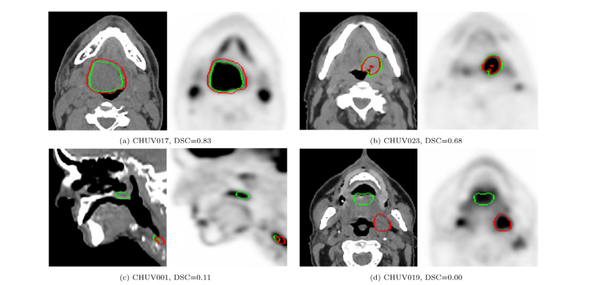
Fig. 2. Examples of results of the winning algorithm (andrei.iantsen (Iantsen et al., 2021b)). The automatic segmentation results (green) and ground truth annotations(red) are displayed on 2D slices of PET (right) and CT (left) images. The reported DSC is computed on the entire image (see Eq. 1). (a), (b) Excellent segmentation results,detecting the GTVt of the primary oropharyngeal tumor localized at the bse of the tongue and discarding the laterocervical lymph nodes despite high FDG uptake onPET. (c) Incorrect segmentation of the top volume at the level of the soft palate; (d) Incorrect segmentation of the smaller volume below the level of the hyoid bone.
图 2. 获胜算法的结果示例(andrei.iantsen (Iantsen等,2021b))。自动分割结果(绿色)和地面真实标注(红色)显示在PET(右侧)和CT(左侧)图像的2D切片上。报告的DSC是在整个图像上计算的(见公式1)。(a) 和 (b) 优秀的分割结果,检测到位于舌根的口咽部原发肿瘤的GTVt,并且尽管PET上FDG摄取量高,也排除了侧颈淋巴结。(c) 在软腭层面的顶部体积分割不正确;(d) 在舌骨下层面的较小体积分割不正确。
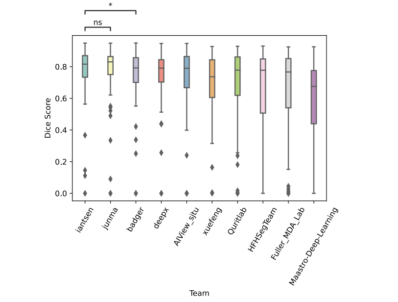
Fig. 3. Box plots of the distribution of the 53 test DSCs for each participant, ordered by decreasing rank.
图 3. 按降序排列的每位参与者的53个测试DSC分布的箱形图。
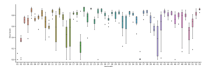
Fig. 4. Box plots of the distribution of DSCs across the 10 participants for each of the 53 patients in the test set.
图 4. 测试集中每位患者的10名参与者DSC分布的箱形图。
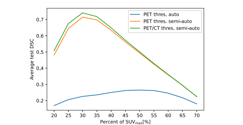
Fig. 5. Segmentation performance of PET thresholding-based method at different percentages of maximum SUV. Three results are reported: the automatic PET threshold, thesemi-automatic PET threshold (indicating the location of the ground truth GTVt), and the semi-automatic PET and CT (for removing the air) threshold.
图 5. 基于不同最大SUV百分比的PET阈值法的分割性能。报告了三个结果:自动PET阈值、半自动PET阈值(指示地面真实GTVt的位置),以及半自动PET和CT(用于去除空气)阈值。
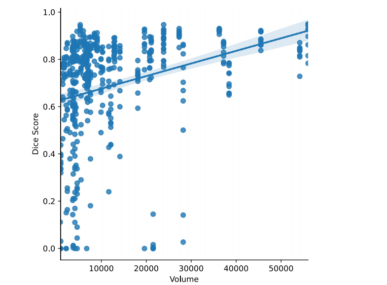
Fig. 6. Scatter plot of DSC vs. tumor volume (voxel count in the VOI) for 10 participants. The corresponding Spearman correlation is 0.43.
图 6。10名参与者中DSC与肿瘤体积(感兴趣区域内的体素计数)的散点图。相应的Spearman相关系数为0.43。
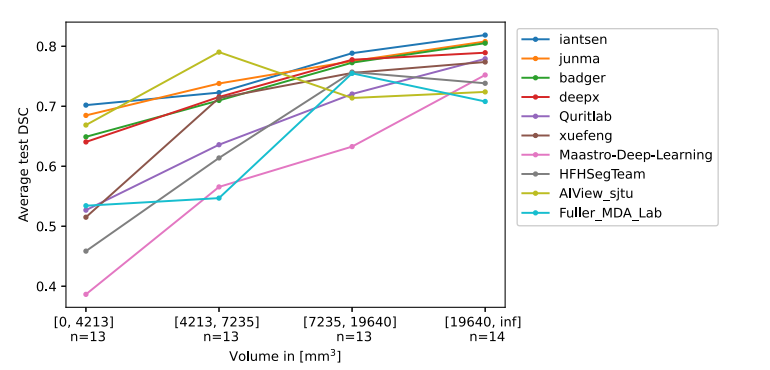
Fig. 7. Average DSC of each team’s algorithm in function of the volume of the tumors. This figure was generated by distributing the 53 test volumes in 4 bins of n =13, 13,13, and 14 each and then computing the average DSC for each bin.
图 7. 每个团队算法的平均DSC与肿瘤体积的关系。此图通过将53个测试体积分布在每个包含13, 13, 13和14个体积的4个区间中,然后计算每个区间的平均DSC生成。
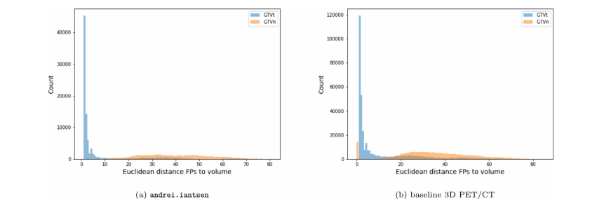
Fig. 8. Histogram of the Euclidean distance of the FP voxels to the closest ground truth GTVt voxel and GTVn voxel. We evaluate here the prediction of the first rankedparticipant (andrei.iantsen) (a) and our baseline 3D PET/CT (b). For comparison, the False Discovery Rate (FDR), i.e. FP/(FP+TP) is 0.15, with 544,343 TPs in (a) and FDR= 0.37 with 621,413 TPs in (b).
图 8. 假阳性体素到最近的地面真实GTVt体素和GTVn体素的欧几里得距离的直方图。这里我们评估第一名参与者(andrei.iantsen)的预测结果(a)和我们的基线3D PET/CT(b)。作为比较,假发现率(FDR),即 FP/(FP+TP) 在 (a) 中为0.15,有544,343个TPs,在 (b) 中为0.37,有621,413个TPs。
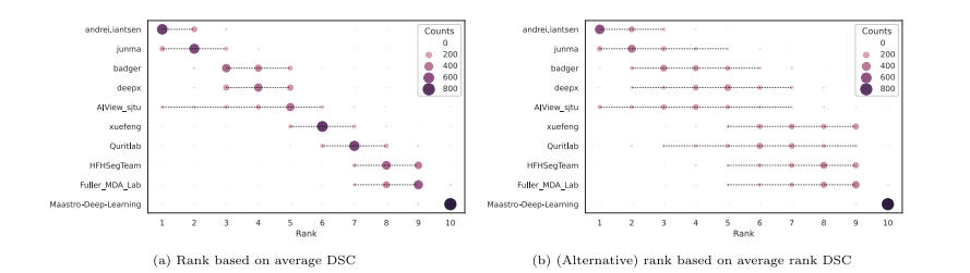
Fig. 9. Ranking robustness against changes in test data. The robustness is assessed by ranking 1000 bootstraps of the test set. The size of the circles is proportional tothe number of times a team obtained the corresponding rank for each bootstrap. The dashed lines represent the confidence intervals at 95% computed from the bootstrapanalysis. The current ranking, i.e. the one used in this challenge, is obtained by averaging the DSCs across all test cases. The alternative ranking is computed by averagingthe rankings of each team across the test cases.
图 9. 排名对测试数据变化的稳健性。通过对测试集的1000个自助样本进行排名来评估稳健性。圆圈的大小与每个自助样本中团队获得相应排名的次数成正比。虚线代表由自助分析计算出的95%置信区间。当前排名,即本挑战赛中使用的排名,是通过平均所有测试案例的DSCs获得的。替代排名是通过平均每个团队在测试案例中的排名计算得出的。
Table
表
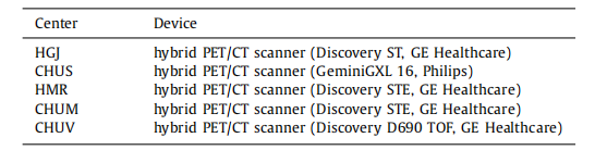
Table 1List of scanners used in the different centers.
表 1 不同中心使用的扫描仪列表。
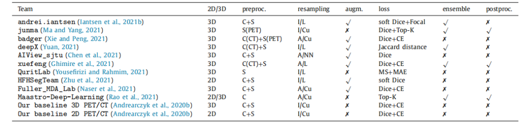
Table 2Summary of the algorithms in terms of main components used: 2D or 3D U-Net, resampling, preprocessing, training or testing data augmentation, loss used for optimization,an ensemble of multiple models for test prediction and postprocessing of the results. We use the following abbreviations for the preprocessing: Clipping (C), Standardization(S), and if it is applied only to one modality, it is specified in parentheses. For the image resampling, we specify whether the algorithms use Isotropic (I) or Anisotropic (A)resampling and Nearest Neighbor (NN), Linear (L), or Cubic (Cu) interpolation. We use the following abbreviation for the losses: Cross-Entropy (CE), Mumford-Shah (MS),and Mean Absolute Error (MAE). More details can be found in the respective participants’ publications.
表 2 关于主要组件使用的算法总结:2D或3D U-Net、重采样、预处理、训练或测试数据增强、用于优化的损失函数、测试预测的多模型集成以及结果的后处理。我们使用以下缩写表示预处理:剪切(C)、标准化(S),如果仅应用于一种模式,则在括号中指定。对于图像重采样,我们指定算法使用的是等距(I)还是非等距(A)重采样以及最近邻(NN)、线性(L)或立方(Cu)插值。我们使用以下缩写表示损失函数:交叉熵(CE)、Mumford-Shah(MS)和平均绝对误差(MAE)。更多详情可以在各参与者的出版物中找到。
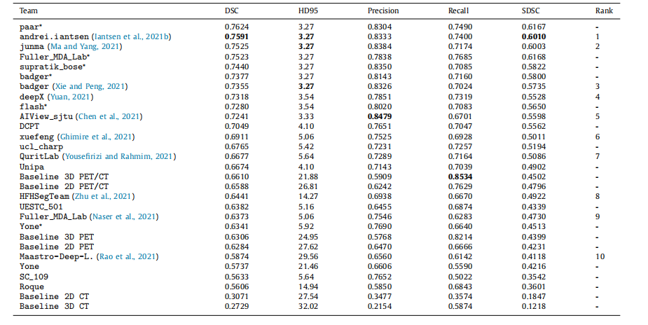
Table 3Summary of the challenge results as of April 2021. The average DSC, precision, recall, SDSC and median HD95 are reported for the baseline algorithms and every team (thebest result of each team). The unit of the HD95 is [mm]. The participant names are reported when no team name was provided. The ranking is only provided for teamsthat presented their method in a paper submission. The post-challenge results are denoted by an asterisk ∗. Bold values represent the best scores for each metric, excludingpost-challenge results since we do not have any information about their method.
表 3截至2021年4月的挑战赛结果总结。报告了基线算法和每个团队(每个团队的最佳结果)的平均DSC、精度、召回率、SDSC和中位HD95。HD95的单位是[毫米]。如果没有提供团队名称,则报告参与者名称。只为提交了方法论文的团队提供排名。挑战赛后的结果由星号∗表示。粗体值代表除挑战赛后结果外每个指标的最佳分数,因为我们没有关于它们方法的任何信息。
这篇关于头颈肿瘤在PET/CT中的分割:HECKTOR挑战赛| 文献速递-深度学习肿瘤自动分割的文章就介绍到这儿,希望我们推荐的文章对编程师们有所帮助!


